V_A <- 4; V_E <- 6; mu <- 50
h2 <- V_A / (V_A + V_E)
make_pop <- function(a) data.frame(a = a, z = mu + a + rnorm(length(a), 0, sqrt(V_E)))
breed <- function(sires, dams, n_off, VA_ms = V_A / 2) {
  s <- sample(nrow(sires), n_off, TRUE); d <- sample(nrow(dams), n_off, TRUE)
  mid <- (sires$a[s] + dams$a[d]) / 2
  out <- make_pop(mid + rnorm(n_off, 0, sqrt(VA_ms)))
  out$mid_z <- (sires$z[s] + dams$z[d]) / 2
  out
}4 The breeder’s equation
Part I measured what selection does within a generation, and stopped where the phenotype stops. A differential of half a standard deviation says that the animals that bred were larger than the animals that did not. It says nothing about whether their offspring will be larger, and a trait can be under strong selection for decades without moving at all if the variation selection acts on is not passed on. The step from selection to evolution needs inheritance, and in quantitative genetics inheritance enters through a single number: the share of the phenotypic variance that is transmitted from parent to offspring in the average way.
This chapter builds that number from a simulated population, uses it to predict the response to selection, and then takes the prediction apart. The prediction holds exactly for one generation under the conditions it assumes, drifts over several generations for a reason that is easy to see in a simulation, and fails completely under a condition that is common in wild populations and invisible in the selection analysis itself.
4.1 Breeding values and heritability
The model behind almost all of quantitative genetics is additive. Each individual’s phenotype is the sum of a breeding value a, the part of its genotype that it passes on in the average way, and a residual e that covers the environment and every non-additive genetic effect:
\[ z = \mu + a + e, \qquad V_P = V_A + V_E . \]
The variance of breeding values is the additive genetic variance V_A, and the narrow-sense heritability is its share of the phenotypic variance, h^2 = V_A / V_P. An offspring receives the average of its parents’ breeding values plus a random term from the shuffling of alleles at meiosis, the Mendelian sampling term, whose variance in a population without inbreeding is half the additive variance (Falconer and Mackay 1996). That is the whole genetic machinery this chapter needs, and it fits in a few lines of R.
The classical way to estimate heritability uses exactly this structure. Regress offspring phenotype on the mean phenotype of the two parents, and the slope estimates h^2: the parents’ phenotypes carry their breeding values diluted by their environments, and the offspring inherit only the breeding values.
set.seed(432)
n <- 5000
sires0 <- make_pop(rnorm(n, 0, sqrt(V_A)))      # n unrelated pairs,
dams0  <- make_pop(rnorm(n, 0, sqrt(V_A)))      # one offspring each
off0 <- make_pop((sires0$a + dams0$a) / 2 + rnorm(n, 0, sqrt(V_A / 2)))
off0$mid_z <- (sires0$z + dams0$z) / 2
po_fit <- lm(z ~ mid_z, data = off0)
po_slope <- unname(coef(po_fit)[2]); po_se <- summary(po_fit)$coefficients[2, 2]
With 5,000 unrelated pairs, one offspring each, the midparent-offspring slope is 0.391 (standard error 0.019) against a true heritability of 0.40, 0.5 standard errors away. The regression works here because the families were bred at random and raised in environments drawn independently of their parents’. In a wild population neither holds for certain. Offspring often share their parents’ territory, diet and nest, and any resemblance they inherit through the environment inflates the slope; Chapter 9 measures how much. For now the simulation keeps the environment honest, so that the arithmetic of the response can be seen on its own.
4.2 One generation: \(R = h^2 S\)
Truncation selection keeps the top fifth of the population by phenotype and breeds them at random. The breeder’s equation predicts the change in mean between the parental and the offspring generations,
\[ R = h^2 S , \]
and it follows from the same regression. The selected parents are S above the mean in phenotype, their expected breeding values are h^2 S above the mean because breeding values regress on phenotypes with slope h^2, and the offspring inherit the average of those breeding values.
set.seed(4321)
keep <- 0.2
pop <- make_pop(rnorm(n, 0, sqrt(V_A)))
chosen <- pop[pop$z >= quantile(pop$z, 1 - keep), ]
S_1 <- mean(chosen$z) - mean(pop$z)
off <- breed(chosen, chosen, n)
R_obs  <- mean(off$z) - mean(pop$z)
R_pred <- h2 * S_1
a_sel  <- mean(chosen$a) - mean(pop$a)     # the selected parents' mean breeding value

one_gen <- function() {
  p0 <- make_pop(rnorm(n, 0, sqrt(V_A)))
  ch <- p0[p0$z >= quantile(p0$z, 1 - keep), ]
  (mean(breed(ch, ch, n)$z) - mean(p0$z)) / (mean(ch$z) - mean(p0$z))
}
n_rep_1 <- 200
ratios <- replicate(n_rep_1, one_gen())
Keeping the top 20 per cent gives a selection differential of 4.362 phenotypic units. The breeder’s equation predicts a response of 1.745. The selected parents have a mean breeding value 1.657 above the population’s, which is the response they can actually pass on, and their offspring move by 1.626; the gap between the last two is Mendelian sampling and the offspring’s own environments, and it is noise. Across 200 replicate experiments the ratio of response to differential averages 0.400, with a Monte Carlo standard error of 0.0012. Only 40 per cent of the phenotypic spread was heritable, so only that share of the selection differential reappears in the next generation. The rest belonged to the environment of the parents and was left behind with them.
4.3 Many generations: the variance does not stay put
Run the same selection for several generations and plot the cumulative response against the cumulative differential. The slope of that line is the realised heritability, the estimate a breeder gets from a selection experiment without any pedigree at all.
set.seed(4322)
n_gen <- 10
pop <- make_pop(rnorm(n, 0, sqrt(V_A)))
base <- mean(pop$z)
rows <- vector("list", n_gen); cS <- 0
for (g in seq_len(n_gen)) {
  chosen <- pop[pop$z >= quantile(pop$z, 1 - keep), ]
  S_g <- mean(chosen$z) - mean(pop$z)
  VA_g <- var(pop$a)
  new <- breed(chosen, chosen, n)
  R_g <- mean(new$z) - mean(pop$z)
  cS <- cS + S_g
  rows[[g]] <- data.frame(gen = g, S = S_g, R = R_g, VA = VA_g,
                          cumS = cS, cumR = mean(new$z) - base)
  pop <- new
}
hist_sel <- do.call(rbind, rows)
h2_real <- unname(coef(lm(cumR ~ 0 + cumS, data = hist_sel))[1])
VA_end  <- var(pop$a)
ratio_first <- hist_sel$R[1] / hist_sel$S[1]
ratio_late  <- mean(tail(hist_sel$R / hist_sel$S, 5))
The realised heritability comes out at 0.360, below the 0.40 built into the base population, and the reason is in the additive variance. It is 4.08 among the first generation’s parents and has fallen to 3.21 among the offspring of the 10th round, with no allele lost and no mutation involved. Truncation selection keeps parents from the upper tail, and parents from the upper tail carry breeding values that are correlated with each other across loci: an individual in the selected tail is there because many of its loci pushed the same way. That correlation between loci, a linkage disequilibrium created by selection itself, reduces the variance of breeding values among the offspring until the loss each generation is balanced by recombination. Bulmer (1971) worked out the equilibrium, and the reduction carries his name. The Mendelian sampling term in the simulation stays at half the base-population additive variance, which is the infinitesimal model’s way of saying that the underlying genetic variation is intact and only its arrangement has changed.
long <- rbind(
  data.frame(x = hist_sel$cumS, y = hist_sel$cumR, panel = "cumulative response"),
  data.frame(x = hist_sel$gen, y = hist_sel$VA, panel = "additive variance"))
long$panel <- factor(long$panel, levels = c("cumulative response", "additive variance"))
ref <- data.frame(panel = factor("cumulative response", levels = levels(long$panel)),
                  slope = h2)
ggplot(long, aes(x, y)) +
  geom_abline(data = ref, aes(slope = slope, intercept = 0),
              colour = te_sage, linetype = "dashed") +
  geom_line(colour = te_forest, linewidth = 0.7) +
  geom_point(colour = te_ink, size = 2) +
  facet_wrap(~ panel, scales = "free",
             labeller = as_labeller(c(`cumulative response` = "cumulative response vs cumulative S",
                                      `additive variance` = "additive variance by generation"))) +
  labs(x = NULL, y = NULL) +
  theme_book()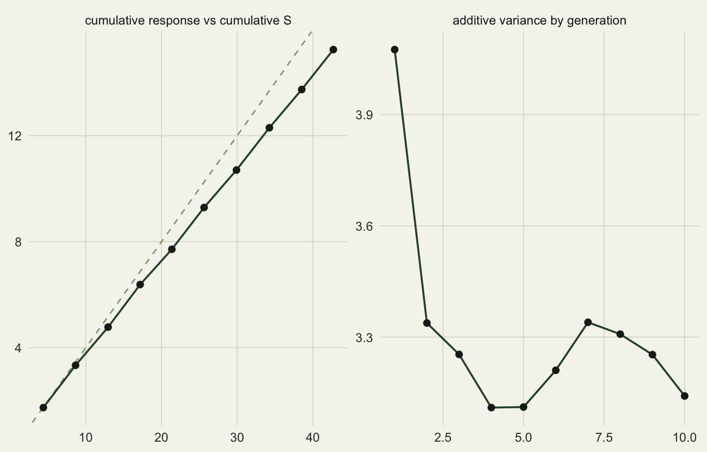
The ratio of response to differential is 0.396 in the first generation and averages 0.353 over the last five. The breeder’s equation is not wrong in any generation; it is exact given the heritability of that generation’s parents. What changes is the heritability, and a prediction that carries the base-population value forward several generations will overestimate the response. Almost all of the loss comes in the first round of selection; after that the variance hovers around its new equilibrium. In the infinitesimal model the disequilibrium decays by half in each generation of random mating once selection stops, so the variance returns about as quickly as it was lost.
4.4 The equation behind the equation
The breeder’s equation is a special case of a more general statement. Robertson (1966) showed that the change in the mean breeding value within a generation is the covariance between breeding value and relative fitness,
\[ R = \operatorname{cov}(a, w), \]
which is the Price equation of Part IV applied to breeding values. The breeder’s equation follows from it only when breeding values are related to fitness through the phenotype and in no other way, so that the regression of a on w passes through z. When that holds, cov(a, w) = h^2 cov(z, w) = h^2 S. When it does not, the two can be very different, and the difference is the most important thing in this chapter.
The standard way for it not to hold is an environmental variable that affects both the trait and fitness. Price, Kirkpatrick and Arnold (1988) made the argument for breeding date in birds, a trait that is heritable and under apparent directional selection, since earlier breeders raise more young, and yet does not evolve. In the version simulated below, an environmental variable such as a female’s condition sets both how early she breeds and how many young she raises. The selection then runs through condition, and the part of breeding date that condition moves is environmental and is not inherited.
set.seed(4323)
n_env <- 20000
cond  <- rnorm(n_env)                         # environmental: territory, food, condition
a_env <- rnorm(n_env, 0, sqrt(V_A))
e_env <- sqrt(V_E) * (0.7 * cond + sqrt(1 - 0.7^2) * rnorm(n_env))
z_env <- mu + a_env + e_env
W_env <- rpois(n_env, exp(0.2 + 0.4 * cond))  # fitness through condition only
w_env <- W_env / mean(W_env)
S_env   <- cov(z_env, w_env)
R_naive <- h2 * S_env
R_true  <- cov(a_env, w_env)
R_true_se <- sd(a_env) * sd(w_env) / sqrt(n_env)
beta_env <- unname(coef(lm(w_env ~ I(z_env / sd(z_env))))[2])
In this population the trait is exactly as heritable as before, h^2 = 0.40, and fitness depends on condition alone. Condition also shifts the environmental part of the trait. The selection differential is 0.719 trait units, and the standardised gradient is 0.227, larger than the median published linear gradient quoted in Chapter 2. The breeder’s equation predicts a response of 0.288 per generation. The true change in mean breeding value, the covariance of breeding value with fitness, is 0.010, with a standard error of about 0.014: no evolution at all.
Nothing in the selection analysis reveals this. The differential is real, the gradient is real, the heritability is real, and their product is meaningless. This is the most likely explanation of the stasis paradox, the observation that heritable traits under measured directional selection in wild populations so often fail to change over decades (Merila and colleagues 2001). Morrissey and colleagues (2010) made the general point, and the remedy follows from Robertson’s form of the equation: estimate the covariance of fitness with breeding values rather than with phenotypes. That needs estimates of breeding values, which need a pedigree, which is where Part III begins. It also needs care, because breeding values predicted from a pedigree are not the true values, and Chapter 10 shows how carrying predicted values into a second analysis goes wrong.
4.5 Where this leaves the equation
The breeder’s equation is exact for one generation when its assumptions hold, and it fails for reasons that can be named. The additive variance changes under selection even without any change in allele frequency. The heritability estimated from relatives is inflated by any environment that relatives share. And the product of a heritability and a phenotypic differential predicts evolution only when fitness is related to breeding values through the phenotype and nothing else, which is precisely what an observational selection analysis cannot check.
All of it has so far concerned one trait. Selection in the field acts on several traits at once and those traits share genes, so a response in one drags the others along. Chapter 5 replaces the heritability with a matrix and the differential with a vector, and finds that the direction selection pushes and the direction a population moves are rarely the same.
References
Falconer DS, Mackay TFC 1996. Introduction to Quantitative Genetics, 4th ed. Longman. ISBN 978-0582243026
Bulmer MG 1971. The American Naturalist 105(943):201-211 (10.1086/282718)
Robertson A 1966. Animal Production 8(1):95-108 (10.1017/S0003356100037752)
Price T, Kirkpatrick M, Arnold SJ 1988. Science 240(4853):798-799 (10.1126/science.3363360)
Merila J, Sheldon BC, Kruuk LEB 2001. Genetica 112-113:199-222 (10.1023/A:1013391806317)
Morrissey MB, Kruuk LEB, Wilson AJ 2010. Journal of Evolutionary Biology 23(11):2277-2288 (10.1111/j.1420-9101.2010.02084.x)