set.seed(434)
beta_true <- 0.15
one_fit <- function(nn, rr) {
  x2 <- rnorm(nn); x1 <- rr * x2 + sqrt(1 - rr^2) * rnorm(nn)
  W  <- rpois(nn, exp(0.2 + beta_true * x1 + beta_true * x2))
  coef(lm(I(W / mean(W)) ~ x1 + x2))[2]
}
vif_of <- function(rr) 1 / (1 - rr^2)
rho_hi <- 0.95; rho_lo <- 0.2
n_study <- 200; n_sims <- 2000
b_hi <- replicate(n_sims, one_fit(n_study, rho_hi))
b_lo <- replicate(n_sims, one_fit(n_study, rho_lo))
wrong_hi <- mean(b_hi < 0); wrong_lo <- mean(b_lo < 0)
sd_ratio <- sd(b_hi) / sd(b_lo)
sd_ratio_expect <- sqrt(vif_of(rho_hi) / vif_of(rho_lo))3 Checking a selection analysis
A selection gradient is a regression coefficient, so everything that can go wrong with a regression can go wrong with it, and a few things go wrong with it in field data far more often than in the textbook examples regression is usually taught with. Traits are strongly correlated because they are aspects of one body. Fitness is a count of offspring or a yes-or-no survival record, never a nicely behaved continuous variable. Traits are measured with error, sometimes a great deal of it. And the traits that were measured are a small, convenient subset of the traits that matter.
This chapter takes those problems one at a time, measures what each does to the estimates of Chapter 1 and Chapter 2, and says what can be done. The first four have remedies inside the data. The last one does not, and it is the one that most often decides whether a selection analysis means what it says.
3.1 Traits that are nearly the same trait
The gradient separates two traits by asking what happens to fitness when one changes and the other does not. When the two are almost perfectly correlated the data contain very few animals in which one changed and the other did not, and the regression has almost nothing to work with. The variance inflation factor, one over one minus the squared multiple correlation of a trait with the others, measures how much that shortage widens the standard error.
Two traits are under equal direct selection, a log-scale effect of 0.15 each, in 2,000 simulated studies of 200 animals. With the traits correlated at 0.20 the estimated gradient on the first trait has the right sign in all but 1.2 per cent of studies. At 0.95 the variance inflation factor is 10.3, the spread of the estimate is 3.0 times wider (the variance inflation factors predict 3.1), and 21.3 per cent of studies report the wrong sign for a trait that is genuinely favoured.
dd <- rbind(data.frame(b = b_lo, corr = sprintf("trait correlation %.2f", rho_lo)),
            data.frame(b = b_hi, corr = sprintf("trait correlation %.2f", rho_hi)))
ggplot(dd, aes(b, fill = corr)) +
  geom_vline(xintercept = 0, colour = te_body, linewidth = 0.4) +
  geom_density(alpha = 0.6, colour = NA) +
  scale_fill_manual(values = c(te_forest, te_gold), name = NULL) +
  labs(x = "estimated gradient on trait 1", y = "density") +
  theme_book()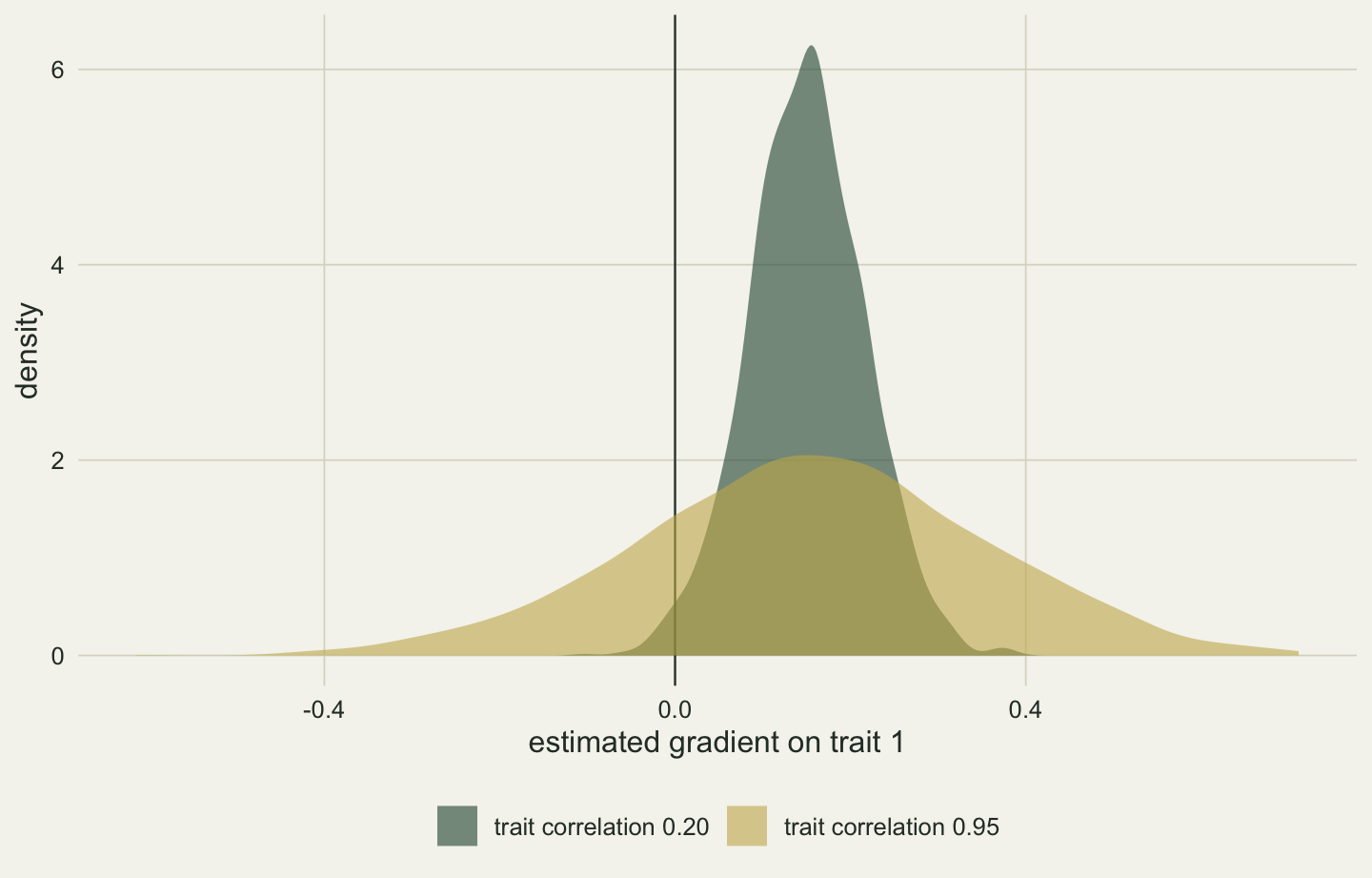
No estimator fixes this, because the information is not in the data. What helps is to look at the variance inflation factors before interpreting anything, and to accept what they imply. If two traits are effectively one measurement, the honest analysis uses one of them, or a composite such as their first principal component, and reports selection on that. The alternative, two gradients with enormous standard errors and opposite signs, invites a story about antagonistic selection that the data never supported.
3.2 Fitness that is not normal
Fitness is a count or a binary outcome, and least squares assumes neither. The point estimate survives this. Lande and Arnold (1983) defined the gradient as the least squares coefficient precisely because it has a meaning, the best linear approximation to the relative fitness surface, whatever the distribution of fitness. What does not survive is the standard error that lm() prints, which assumes constant, normal residual variance. Count data have a variance that rises with the mean, so the printed standard error is wrong even when the estimate is right. Resampling individuals gives an interval that does not lean on that assumption (Mitchell-Olds and Shaw 1987).
set.seed(505)
n_b <- 500
z  <- rnorm(n_b)
Wc <- rpois(n_b, exp(0.1 + 0.4 * z)); wc <- Wc / mean(Wc)
m_c <- lm(wc ~ z)
se_lm <- summary(m_c)$coefficients["z", 2]
boot <- replicate(2000, { i <- sample(n_b, replace = TRUE)
  ww <- Wc[i] / mean(Wc[i]); coef(lm(ww ~ z[i]))[2] })
se_boot <- sd(boot)
The gradient is 0.385. Its printed standard error is 0.040 and its bootstrap standard error 0.045, so the model-based interval is too narrow by 11 per cent. Note that each bootstrap sample recomputes relative fitness from its own mean: the mean of fitness is estimated from the same data, and leaving it fixed understates the uncertainty a little further.
Binary fitness raises a different problem, because the natural model for it is not linear at all. A logistic regression of survival on a trait is the right model for the data, and its coefficient is not a selection gradient. The logistic coefficient is a slope on the log-odds scale; the gradient is the average slope of relative survival. Janzen and Stern (1998) gave the conversion: average the derivative of the fitted survival probability over the individuals, and divide by mean survival.
set.seed(606)
n_s <- 800
zs <- rnorm(n_s)
alive <- rbinom(n_s, 1, plogis(0.4 + 0.8 * zs))
w_s <- alive / mean(alive)
b_ols   <- unname(coef(lm(w_s ~ zs))[2])
fit_lg  <- glm(alive ~ zs, family = binomial)
b_logit <- unname(coef(fit_lg)[2])
p_hat   <- fitted(fit_lg)
b_js    <- mean(b_logit * p_hat * (1 - p_hat)) / mean(alive)
In a sample of 800 animals with a survival rate of 58 per cent, the logistic coefficient is 0.674. Converted to the relative fitness scale it becomes 0.255, and the least squares gradient on relative survival is 0.256. The converted and the direct estimates agree closely; the raw logistic coefficient is 2.6 times either of them. Both routes are defensible, and the logistic one has the advantage that its fitted surface never predicts a survival probability outside zero and one. What is not defensible is to put a logistic coefficient into a table of selection gradients, or into a breeder’s equation, as though it were one.
3.3 The gap between differential and gradient
The difference between a trait’s differential and its gradient is not a nuisance to be explained away. By the identity of Chapter 1 it is exactly the indirect selection the trait received through its correlations with the other traits in the model, so it is a measurement in its own right, and a large gap marks a trait that is being carried rather than selected.
set.seed(607)
n_g <- 400
rho_g <- 0.7
t2 <- rnorm(n_g); t1 <- rho_g * t2 + sqrt(1 - rho_g^2) * rnorm(n_g)
Wg <- rpois(n_g, exp(0.2 + 0.35 * t2)); wg <- Wg / mean(Wg)
S_g <- c(cov(t1, wg), cov(t2, wg))
b_g <- drop(solve(cov(cbind(t1, t2))) %*% S_g)
gap <- S_g - b_g
In a sample of 400 with a passenger trait correlated at 0.70 with the real target, the passenger has a differential of 0.192 and a gradient of 0.007, a gap of 0.185; the target has a differential of 0.290, a gradient of 0.312 and a gap of -0.022. Reporting both numbers for every trait costs one extra column in a table and lets a reader see at once which traits are selected and which are travelling with them. Reporting only the differential hides the indirect selection; reporting only the gradient hides how much selection the trait actually experienced, which is the quantity that enters the response in the next chapter.
3.4 Traits measured with error
Measurement error in a single trait is familiar: it attenuates the slope towards zero, by a factor equal to the reliability of the measurement, the share of its variance that is real. With several correlated traits the effect is less familiar and worse. The regression uses the other traits to stand in for the part of the noisy trait it cannot see, so the selection that attenuation removes from the noisy trait does not disappear. It moves to whichever correlated trait was measured more precisely.
set.seed(608)
n_e <- 20000
rel <- 0.6                       # reliability of the noisy measurement of the target
tru2 <- rnorm(n_e)
obs1 <- 0.6 * tru2 + sqrt(1 - 0.6^2) * rnorm(n_e)       # passenger, measured exactly
obs2 <- sqrt(rel) * tru2 + sqrt(1 - rel) * rnorm(n_e)   # target, measured with error
We <- rpois(n_e, exp(0.2 + 0.35 * tru2)); we <- We / mean(We)
b_true <- coef(lm(we ~ obs1 + tru2))[2:3]
b_err  <- coef(lm(we ~ obs1 + obs2))[2:3]
The target trait is recorded with a reliability of 0.60, which is not pessimistic for a single behavioural score (the average repeatability of behaviour across published studies is lower still; Bell and colleagues 2009), and the passenger is measured exactly. With the true values of the target in the model, the gradients are 0.001 on the passenger and 0.345 on the target. With the noisy measurement in its place they become 0.110 and 0.217. The target has lost selection, as expected, and the passenger, which the simulation gave no effect at all, has gained a gradient large enough to be reported as a finding. A large sample does nothing to prevent this; the numbers above come from 20,000 animals.
There are two remedies and both need extra data. Repeated measurements of the noisy trait give an estimate of its reliability, which can be used to correct the covariance matrix before inverting it, and they also make it possible to fit the trait as a latent variable in a mixed model. Chapter 6 builds that machinery. Short of it, the defensible report states the reliability of each trait, and treats a gradient on a precisely measured trait that correlates with a poorly measured one as suspect until shown otherwise.
3.5 The trait that was not measured
The last check is the one no diagnostic can perform. As Chapter 1 warned, an unmeasured trait that affects fitness and correlates with a measured one hands its selection to the measured trait. The arithmetic is the omitted variable bias of any regression: the gradient on the measured trait becomes its own gradient plus the missing trait’s gradient multiplied by the regression of the missing trait on the measured one.
set.seed(609)
n_o <- 20000
cond <- rnorm(n_o)                                   # unmeasured: condition
rho_o <- 0.5
size <- rho_o * cond + sqrt(1 - rho_o^2) * rnorm(n_o)   # measured: size, no own effect
Wo <- rpois(n_o, exp(0.2 + 0.30 * cond)); wo <- Wo / mean(Wo)
b_full <- coef(lm(wo ~ size + cond))
b_size <- unname(coef(lm(wo ~ size))[2])
b_pred <- unname(b_full["size"] + b_full["cond"] * coef(lm(cond ~ size))[2])
Here fitness depends on condition, which was not recorded, and not on size, which was. Condition and size are correlated at 0.50. With condition in the model the gradient on size is 0.002. Without it the gradient on size is 0.152, and the omitted variable formula predicts 0.152. Nothing in the fitted model signals the problem. The variance inflation factor is one because there is only one trait, and a bootstrap interval measures sampling error, which this is not: with more data the interval narrows around the wrong value.
Condition is the standard example for a reason. Animals in good condition are often larger, breed earlier and survive better, and the environment that produced the good condition does all three at once without any causal path from size to fitness. When the missing variable is environmental in this way, the damage is not confined to the estimate of direct selection. It reaches the prediction of evolutionary change too, because a covariance between a trait and fitness that runs through the environment will not be passed to the next generation. That is the subject of Chapter 4, where it resolves a long-standing puzzle about why heritable traits under measured selection so often fail to evolve.
The defences are all outside the regression. The strongest is experimental manipulation of the trait, which breaks its correlation with everything else. Another is to measure the obvious confounders, condition, age, territory quality, and put them in the model even when they are not the traits of interest. A third, which needs a pedigree, is to estimate the covariance of fitness with breeding values rather than with phenotypes, so that environmental routes drop out by construction; Morrissey and colleagues (2010) made the case for that approach, and it becomes available in Part III.
3.6 A checklist
Before a selection gradient is interpreted: compute the variance inflation factors and act on large ones; take standard errors from resampling, not from lm(); if fitness is binary and a logistic model was fitted, convert its coefficient before reporting it as a gradient; report the differential and the gradient side by side; state the reliability of each trait and look hard at gradients on well measured traits that correlate with poorly measured ones; and list the plausible unmeasured confounders, with what was done about each. The last item has no computational answer, which is why it belongs in the paper as a sentence rather than in the analysis as a test.
References
Lande R, Arnold SJ 1983. Evolution 37(6):1210-1226 (10.1111/j.1558-5646.1983.tb00236.x)
Mitchell-Olds T, Shaw RG 1987. Evolution 41(6):1149-1161 (10.1111/j.1558-5646.1987.tb02457.x)
Janzen FJ, Stern HS 1998. Evolution 52(6):1564-1571 (10.1111/j.1558-5646.1998.tb02237.x)
Bell AM, Hankison SJ, Laskowski KL 2009. Animal Behaviour 77(4):771-783 (10.1016/j.anbehav.2008.12.022)
Morrissey MB, Kruuk LEB, Wilson AJ 2010. Journal of Evolutionary Biology 23(11):2277-2288 (10.1111/j.1420-9101.2010.02084.x)