w_true   <- 1.2        # width of the Gaussian surface, in trait SD
n_plant  <- 8000
mu_seed  <- 12

set.seed(8201)
z_fl   <- rnorm(n_plant)
surf   <- exp(-z_fl^2 / (2 * w_true^2))
seeds  <- rpois(n_plant, mu_seed * surf)
w_rel  <- seeds / mean(seeds)

m_quad  <- lm(w_rel ~ z_fl + I(z_fl^2))
b_hat   <- unname(coef(m_quad)[2])
c_raw   <- unname(coef(m_quad)[3])
c_se    <- summary(m_quad)$coefficients[3, 2]
gam_hat <- 2 * c_raw
P_tr    <- var(z_fl)
gam_theory <- -1 / (w_true^2 + P_tr)2 The shape of selection
The gradient of Chapter 1 is a slope, and a slope describes selection that moves a trait. Much of the selection that field studies set out to find does something else. Plants that flower too early meet a frost and plants that flower too late run out of pollinators; birds with very short and very long wings both die in a hard winter; in each case the survivors have much the same mean as the population they came from, and the directional gradient is close to zero. What differs is how quickly fitness falls away on either side of the middle, and that is a statement about the curvature of the fitness surface rather than its slope.
This chapter adds the second-order terms to the selection regression. The arithmetic is short, but three things about it catch out a large share of published analyses: a factor of two in the definition, an optimum that does not sit where the trait mean does, and a correlation between traits that makes a saddle look like curvature along a single axis. A fourth problem is not arithmetic at all: at the strengths that the published record suggests are typical, the curvature is the part of selection a field study of ordinary size mostly fails to see.
2.1 The second-order expansion, and the half in front of it
Lande and Arnold (1983) extended the regression of relative fitness on the traits to second order:
\[ w = \alpha + \sum_i \beta_i z_i + \frac{1}{2} \sum_i \sum_j \gamma_{ij} z_i z_j + \varepsilon . \]
The coefficients gamma form a symmetric matrix of quadratic selection gradients. The diagonal entries measure curvature along each trait, negative for a hump (stabilising selection) and positive for a bowl (disruptive selection). The off-diagonal entries measure correlational selection, which favours particular combinations of traits. The same argument that made beta the average slope in Chapter 1 makes gamma the average curvature: for multivariate normal traits the matrix equals the expected second derivative of the relative fitness surface over the population.
The one half in front of the double sum is the half that stands in front of every second derivative in a Taylor expansion, and it is the source of the first error. A single trait contributes the term 0.5 * gamma * z^2, so the coefficient that lm() reports for I(z^2) estimates half the gradient, and the gradient is twice the printed number. For two different traits the double sum visits the pair twice, as ij and as ji; the two halves add to one, and the coefficient of the product z1:z2 is already the gradient. Squared terms are doubled, cross-products are not. Stinchcombe and colleagues (2008) audited a set of later papers and found that most of them had skipped the doubling, and that many gave a reader no way to tell.
Here is a surface where the answer is known. Flowering date is standardised, seed set is Poisson around a Gaussian fitness function with its peak at the mean date, and the sample is far larger than any study of this kind so that the arithmetic, not the sampling error, is what shows.
The linear gradient is -0.003, as it should be when the optimum sits at the mean. The coefficient of the squared term is -0.2059 (standard error 0.0028), and the quadratic gradient is therefore -0.4117. For this surface and this trait distribution the value it ought to take can be written down, -0.4108, as the next section shows; the doubled estimate lands on it, and the printed coefficient misses it by a factor of two.
bins <- cut(z_fl, seq(-3.3, 3.3, by = 0.3))
bin_dat <- data.frame(z = tapply(z_fl, bins, mean), w = tapply(w_rel, bins, mean),
                      k = tapply(w_rel, bins, length))
bin_dat <- bin_dat[!is.na(bin_dat$z) & bin_dat$k >= 20, ]
grid_z <- data.frame(z_fl = seq(-3.3, 3.3, length.out = 300))
curves <- data.frame(
  z = rep(grid_z$z_fl, 2),
  y = c(exp(-grid_z$z_fl^2 / (2 * w_true^2)) / mean(surf), predict(m_quad, grid_z)),
  curve = rep(c("true surface", "fitted quadratic"), each = nrow(grid_z)))
ggplot(bin_dat, aes(z, w)) +
  geom_hline(yintercept = 0, colour = te_line) +
  geom_point(colour = te_ink, size = 2) +
  geom_line(data = curves, aes(z, y, colour = curve), linewidth = 0.9) +
  scale_colour_manual(values = c("true surface" = te_forest,
                                 "fitted quadratic" = te_rust), name = NULL) +
  labs(x = "flowering date (standardised)", y = "relative fitness") +
  theme_book()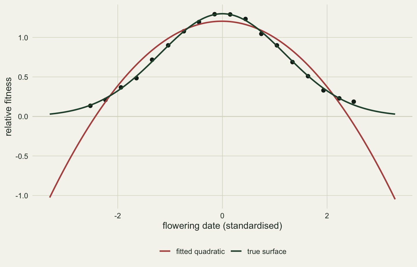
The figure is also a reminder of what the quadratic is. It follows the surface where the data are dense and leaves it in the tails, eventually predicting negative fitness. A second-order regression does not claim that the surface is a parabola; it claims that a parabola is a fair local description over the range the traits occupy.
2.2 From a gradient to a width
A quadratic gradient is hard to picture. The width of the fitness surface, the distance in trait units over which fitness falls away, is easy to picture, and for a Gaussian surface the two are linked exactly. Take a surface of width omega with its peak at theta, and a normal trait with variance P. The product of the trait density and the fitness function is another normal density, and carrying its mean and variance through the two gradients gives
\[ \beta = \frac{\theta}{\omega^2 + P}, \qquad \gamma = \frac{\theta^2 - (\omega^2 + P)}{(\omega^2 + P)^2} = \beta^2 - \frac{1}{\omega^2 + P}. \]
Solving the second form for the width,
\[ \omega = \sqrt{\frac{1}{\beta^2 - \gamma} - P} , \]
which reduces to the recipe usually quoted, sqrt(-1 / gamma - P), only when beta is zero. The P inside the root is a reminder that the regression measures curvature averaged over where the trait actually lies. A widely spread trait samples the flanks of the surface as well as its peak, and the average curvature it reports is gentler than the curvature at the top.
omega_dbl <- sqrt(-1 / gam_hat - P_tr)
omega_raw <- sqrt(-1 / c_raw - P_tr)
infl_fit    <- omega_raw / omega_dbl
infl_closed <- sqrt(2 + P_tr / w_true^2)
The doubled gradient gives a width of 1.198 trait standard deviations against a true width of 1.20. The undoubled coefficient gives 1.966, a surface 64 per cent wider than the one the plants experienced. The size of that error does not depend on the particular sample. Both widths are functions of the same fitted number, so it cancels from their ratio, which is sqrt(2 + P / omega^2): 1.640 here against 1.641 from the fits. The ratio can approach the square root of two when selection is weak and the surface is wide, and never falls below it. Forgetting the doubling therefore overstates the width of every Gaussian surface by at least 41 per cent.
2.3 An optimum away from the mean
A simulation can put the optimum at the trait mean. A field population rarely obliges, because a population whose optimum has moved, with a new climate or a new predator, is exactly the kind a study is likely to be about. Moving the peak adds a slope at the mean, and the identity above says what the slope does to the curvature: gamma rises by beta squared, whatever the width. The check below builds three surfaces of the same width with their peaks at increasing distances from the mean, fits each with a very large sample, and recovers the width both ways. The reference strengths are the medians of the absolute gradients compiled by Kingsolver and colleagues (2001) from the published literature.
b_lit <- 0.16          # median absolute linear gradient, Kingsolver et al. 2001
g_lit <- -0.10         # median absolute quadratic gradient, taken as stabilising
gam_at   <- function(om, bb, pp) bb^2 - 1 / (pp + om^2)
om_naive <- function(gg, pp) sqrt(-1 / gg - pp)
om_joint <- function(bb, gg, pp) sqrt(1 / (bb^2 - gg) - pp)

theta_set <- c(0, 0.8, 1.6)
n_big <- 400000
set.seed(8204)
fits <- vapply(theta_set, function(th) {
  z  <- rnorm(n_big, 0, sqrt(P_tr))
  wr <- exp(-(z - th)^2 / (2 * w_true^2)); wr <- wr / mean(wr)
  cf <- coef(lm(wr ~ z + I(z^2)))
  c(unname(cf[2]), 2 * unname(cf[3]))
}, numeric(2))
gam_pred <- gam_at(w_true, theta_set / (w_true^2 + P_tr), P_tr)
dev_max  <- max(abs(fits[2, ] - gam_pred))
om_back  <- om_joint(fits[1, ], fits[2, ], P_tr)

om_lit   <- om_naive(g_lit, P_tr)                    # width a centred reading implies
err_med  <- om_naive(gam_at(om_lit, b_lit, P_tr), P_tr) / om_lit
err_strong <- om_naive(gam_at(om_lit, 1.5 * b_lit, P_tr), P_tr) / om_lit
b_flip_wide   <- 1 / sqrt(P_tr + om_lit^2)
b_flip_narrow <- 1 / sqrt(P_tr + w_true^2)
For peaks at 0.00, 0.80 and 1.60 standard deviations from the mean, the fitted quadratic gradients match the closed form to within 0.0017, and the joint recipe returns widths of 1.204, 1.198 and 1.204 against 1.20 every time. The short recipe fails on the third surface outright: its quadratic gradient is positive, and a positive gradient has no width.
The literature medians show what this costs in practice. Read as a centred surface, a quadratic gradient of -0.10 implies a width of 3.00 standard deviations. If the population in fact sits on the slope of such a surface, far enough from the peak for its linear gradient to reach the median of 0.16, the short recipe overstates the width by 18 per cent; at one and a half times the median it overstates it by 58 per cent. The error runs in the same direction as the missing doubling, so the two compound. Beyond a linear gradient of 0.316 the quadratic gradient of that wide surface changes sign, and a population under purely stabilising selection is reported as under disruptive selection. The narrow surface resists longer, to 0.641: the flatter the true surface, the less directional selection it takes to turn a hill into an apparent valley.
b_seq <- seq(0, 0.7, length.out = 260)
dd <- expand.grid(bb = b_seq, om = c(w_true, om_lit))
dd$gam <- gam_at(dd$om, dd$bb, P_tr)
dd$surface <- sprintf("true width %.1f", dd$om)
d_ratio <- subset(dd, gam < 0)
d_ratio$y <- om_naive(d_ratio$gam, P_tr) / d_ratio$om
d_ratio <- subset(d_ratio, y <= 4)
long <- rbind(
  data.frame(bb = d_ratio$bb, y = d_ratio$y, surface = d_ratio$surface,
             panel = "recovered width / true width"),
  data.frame(bb = dd$bb, y = dd$gam, surface = dd$surface,
             panel = "quadratic gradient"))
long$panel <- factor(long$panel, levels = c("recovered width / true width",
                                            "quadratic gradient"))
ref <- data.frame(panel = factor(levels(long$panel), levels = levels(long$panel)), y0 = c(1, 0))
ggplot(long, aes(bb, y, colour = surface)) +
  geom_hline(data = ref, aes(yintercept = y0), colour = te_line) +
  geom_vline(xintercept = b_lit, colour = te_gold, linetype = "22") +
  geom_line(linewidth = 0.9) +
  facet_wrap(~ panel, scales = "free_y") +
  scale_colour_manual(values = c(te_forest, te_rust), name = NULL) +
  labs(x = "linear selection gradient", y = NULL) +
  theme_book()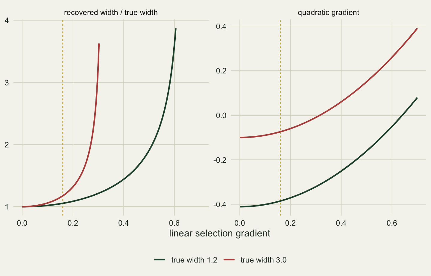
2.4 Curvature along axes nobody measured
With two or more traits the quadratic gradients form a matrix, and the matrix describes curvature along whatever axes the observer chose to measure. The surface has no reason to curve along those axes. Consider two correlated traits, body size and flowering date, on a surface with no curvature along either of them and a single nonlinear term in their product: large late plants and small early plants do well, the mismatched combinations do badly.
n_pair <- 4000
rho    <- 0.6
g12    <- 0.30
set.seed(8203)
z_size <- rnorm(n_pair)
z_date <- rho * z_size + sqrt(1 - rho^2) * rnorm(n_pair)
surf2  <- 1 + g12 * (z_size * z_date - rho)
off    <- rpois(n_pair, 12 * pmax(surf2, 0.05))
w2     <- off / mean(off)

m_one   <- lm(w2 ~ z_size + I(z_size^2))
g11_one <- 2 * unname(coef(m_one)[3])
t_one   <- summary(m_one)$coefficients[3, 3]
g11_expect <- 2 * rho * g12

m_full <- lm(w2 ~ z_size + z_date + I(z_size^2) + I(z_date^2) + z_size:z_date)
cf <- coef(m_full); tb <- summary(m_full)$coefficients
Gam <- matrix(c(2 * cf[["I(z_size^2)"]], cf[["z_size:z_date"]],
                cf[["z_size:z_date"]], 2 * cf[["I(z_date^2)"]]), 2,
              dimnames = list(c("size", "date"), c("size", "date")))
t_sq  <- tb[c("I(z_size^2)", "I(z_date^2)"), 3]
t_12  <- tb["z_size:z_date", 3]
eg    <- eigen(Gam)
ax1   <- eg$vectors[, 1] * sign(eg$vectors[1, 1])
ang1  <- atan2(ax1[2], ax1[1]) * 180 / pi
Fitted on size alone, the quadratic gradient is 0.367 with a t value of 40. Anyone reading that number in the usual way would report strong disruptive selection on body size. The true curvature along the size axis is zero.
The illusion has an exact size. A regression on size alone averages over flowering date, and for standardised traits the expected date given size is the correlation times size; the product term therefore leaves g12 * rho * size^2 in the fitted surface, and doubling gives 0.36 against the 0.367 fitted. The apparent curvature is the correlational gradient times the trait correlation, counted twice.
The full model puts the curvature back where it belongs. The two squared terms give gradients of -0.019 and 0.004, with t values of -1.69 and 0.46, and the cross-product gives 0.305 against the 0.30 built in, with a t value of 36. Neither squared term is distinguishable from zero, though the first comes closer than a true zero comfortably should; fitting the right model does not promise a clean answer on every term.
Phillips and Arnold (1989) pointed out that the diagonal of the matrix is the wrong place to look for stabilising or disruptive selection at all. The eigenvalues of the matrix are the curvatures along the axes the surface actually has, and their signs classify it. Here they are +0.298 and -0.312, against plus and minus 0.30 in the generating surface: one positive and one negative, a saddle. The axis of positive curvature lies at 46 degrees to the size axis, the combination of large and late. The single-trait fit saw that positive eigenvalue through the correlation, gave all of it to body size, and returned a curvature 1.2 times the strongest curvature the real surface has in any direction.
pg <- expand.grid(z_size = seq(-2.6, 2.6, length.out = 90),
                  z_date = seq(-2.6, 2.6, length.out = 90))
pg$w <- predict(m_full, pg)
ends <- 2.4 * eg$vectors
seg <- data.frame(x = -ends[1, ], y = -ends[2, ], xe = ends[1, ], ye = ends[2, ])
ggplot(pg, aes(z_size, z_date)) +
  geom_contour(aes(z = w, colour = after_stat(level)), bins = 14, linewidth = 0.5) +
  geom_segment(data = seg, aes(x = x, y = y, xend = xe, yend = ye),
               colour = te_ink, linetype = "22", linewidth = 0.6) +
  scale_colour_gradient(low = te_rust, high = te_forest, name = "fitted w") +
  coord_equal() +
  labs(x = "body size (standardised)", y = "flowering date (standardised)") +
  theme_book()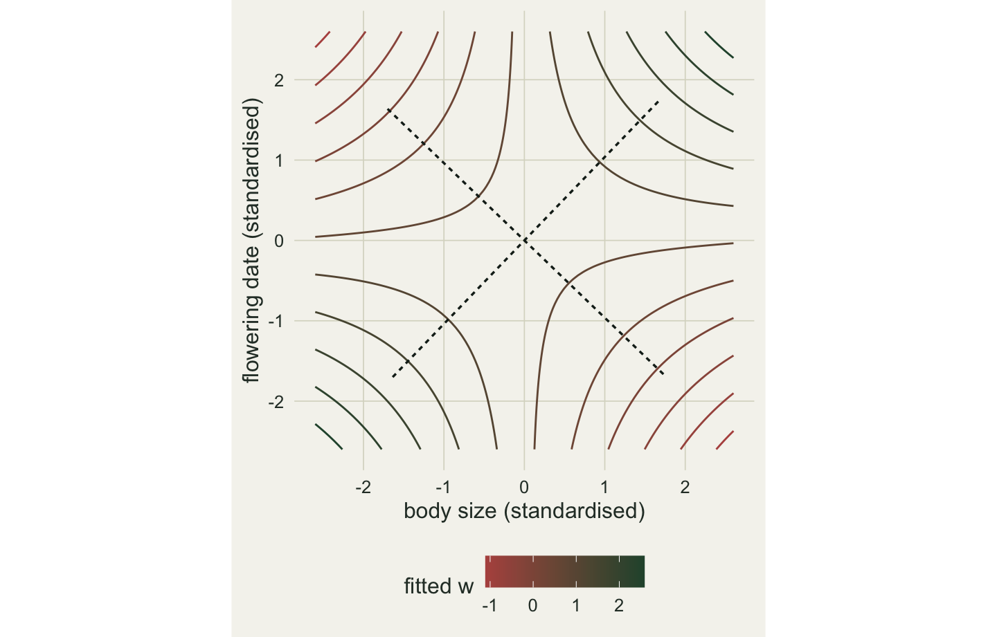
2.5 How often curvature can be seen
Every estimate so far came from samples no field study will have. The practical question is how often a study of ordinary size detects each kind of selection at the strengths the literature reports. The generating surface below has the median linear gradient and a quadratic gradient at the median, with offspring counts near replacement. There is a complication in choosing that quadratic value, and it follows from the first section of this chapter. If most of the estimates behind the compiled median were never doubled, as the audit of Stinchcombe and colleagues suggests of the papers it examined, the true median curvature is nearer twice the compiled number. The simulation runs at both values, because the compiled figure alone cannot say which is right.
n_grid <- c(100, 200, 500, 1000, 2000)
n_rep  <- 6000
g_dbl  <- 2 * g_lit
one_study <- function(nn, gg) {
  z  <- rnorm(nn)
  sf <- 1 + b_lit * z + 0.5 * gg * (z^2 - 1)
  o  <- rpois(nn, 1.2 * pmax(sf, 0.05))
  wr <- o / mean(o)
  ct <- summary(lm(wr ~ z + I(z^2)))$coefficients
  c(ct[2, 4], ct[3, 4], 2 * ct[3, 1])
}
sweep <- function(gg) lapply(n_grid, function(nn)
  vapply(seq_len(n_rep), function(k) one_study(nn, gg), numeric(3)))
hit <- function(runs, i) vapply(runs, function(m) mean(m[i, ] < 0.05), 0)

set.seed(8202); runs_lit <- sweep(g_lit)
set.seed(8222); runs_dbl <- sweep(g_dbl)
set.seed(8212); runs_null <- vapply(seq_len(n_rep), function(k) one_study(n_grid[1], 0), numeric(3))
det <- data.frame(n = n_grid, lin = hit(runs_lit, 1),
                  quad = hit(runs_lit, 2), quad_dbl = hit(runs_dbl, 2))
null_rate <- mean(runs_null[2, ] < 0.05)
small     <- runs_lit[[1]]
sig       <- small[2, ] < 0.05
g_sig     <- mean(abs(small[3, sig]))
wrong_sig <- mean(small[3, sig] > 0)
n_ratio   <- (b_lit / (abs(0.5 * g_lit) * sqrt(2)))^2
At 100 individuals the linear term is detected in 38 per cent of 6,000 simulated studies and the quadratic term in 9.0 per cent, against a false-positive rate of 4.8 per cent when the true curvature is zero. At 500 individuals the quadratic term is found 39 per cent of the time if the compiled median is right and 93 per cent of the time if the doubled value is; only at 2,000 does the first reach 94 per cent. The gap between the two terms is arithmetic. The linear coefficient multiplies z, whose standard deviation is one; the quadratic coefficient multiplies z^2, whose standard deviation is the square root of two, and it is half the gradient. At the compiled medians equal power needs 5.1 times as many individuals for the curvature as for the slope.
Low power has a second consequence that matters more for reading the literature than for planning a study. Among the small studies that did find significant curvature, the mean absolute quadratic gradient is 0.314, 3.1 times the value that generated the data, and 3.3 per cent of them have the wrong sign. Significance at 100 individuals selects the replicates in which noise pushed the estimate away from zero. A published quadratic gradient from a small study is best read as an upper bound, and the published record as a whole as a sample of the curvature that was large enough to report.
lab_q <- sprintf("quadratic, gamma = %.2f", c(g_dbl, g_lit))
det_long <- data.frame(n = rep(det$n, 3), rate = c(det$lin, det$quad_dbl, det$quad),
                       term = factor(rep(c("linear", lab_q), each = nrow(det)),
                                     levels = c("linear", lab_q)))
ggplot(det_long, aes(n, rate, colour = term)) +
  geom_hline(yintercept = null_rate, colour = te_line, linetype = "dashed") +
  geom_line(linewidth = 0.9) + geom_point(size = 2.4) +
  scale_x_log10(breaks = n_grid) + scale_y_continuous(limits = c(0, 1)) +
  scale_colour_manual(values = c(te_forest, te_gold, te_rust), name = NULL) +
  labs(x = "individuals in the study", y = "share of studies detecting the term") +
  theme_book()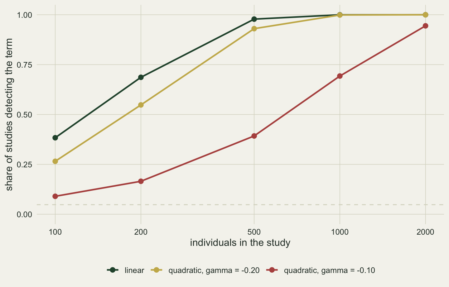
2.6 What to report, and what the quadratic cannot say
The reporting rules follow directly from the arithmetic. State that squared coefficients were doubled, in the methods, because a reader cannot tell from a table. Report the whole matrix with its standard errors and the sample size, including the terms that missed significance, since a later synthesis needs the misses as much as the hits. Report the eigenvalues and eigenvectors, because only they classify the surface. When a width is quoted, compute it from both gradients and give the trait variance alongside.
The limits are of a different kind. The quadratic is a local approximation, and the canonical axes it finds live in the space of the traits that were measured; an unmeasured trait correlated with both would rotate the axes and could flip the sign of an eigenvalue with nothing in the data to show it. The exact width results assume a Gaussian surface and normal traits, and a skewed trait breaks them in the same way that it broke the reading of beta in Chapter 1. The detection rates are a ceiling: real fitness data are more overdispersed than Poisson, and real studies spend their degrees of freedom on more traits than one. And fitness in a single episode is not lifetime fitness; curvature in fecundity can be undone by curvature in survival. Blows and Brooks (2003) made the broader case that a study rarely supports as many dimensions of nonlinear selection as it has traits.
A further problem appears when the trait itself is not measured once but estimated, as a behavioural score averaged over repeated tests usually is. If the number of tests an animal receives depends on how long it lives, the spread of its score depends on its fitness, and the quadratic gradient can report curvature that does not exist. That case needs the machinery of repeatability and random effects, and it is taken up in Chapter 10 once that machinery is in place. The next chapter stays with the linear regression and asks what else can quietly break it.
References
Lande R, Arnold SJ 1983. Evolution 37(6):1210-1226 (10.1111/j.1558-5646.1983.tb00236.x)
Stinchcombe JR, Agrawal AF, Hohenlohe PA, Arnold SJ, Blows MW 2008. Evolution 62(9):2435-2440 (10.1111/j.1558-5646.2008.00449.x)
Kingsolver JG, Hoekstra HE, Hoekstra JM, Berrigan D, Vignieri SN, Hill CE, Hoang A, Gibert P, Beerli P 2001. The American Naturalist 157(3):245-261 (10.1086/319193)
Phillips PC, Arnold SJ 1989. Evolution 43(6):1209-1222 (10.1111/j.1558-5646.1989.tb02569.x)
Blows MW, Brooks R 2003. The American Naturalist 162(6):815-820 (10.1086/378905)