library(ggplot2)

te_paper  <- "#f5f4ee"
te_ink    <- "#16241d"
te_body   <- "#2c3a31"
te_forest <- "#275139"
te_rust   <- "#b5534e"
te_gold   <- "#c9b458"
te_line   <- "#dad9ca"

theme_datasheet <- function() {
  theme_minimal(base_size = 12) +
    theme(plot.background  = element_rect(fill = te_paper, colour = NA),
          panel.background = element_rect(fill = te_paper, colour = NA),
          panel.grid.major = element_line(colour = te_line, linewidth = 0.3),
          panel.grid.minor = element_blank(),
          text             = element_text(colour = te_body),
          plot.title       = element_text(colour = te_ink, face = "bold"),
          plot.subtitle    = element_text(colour = te_body),
          axis.text        = element_text(colour = te_body))
}Zeros and ones in beta regression
R
beta regression
proportions
censoring
simulation
ecology tutorial
The usual squeeze for exact zeros and ones makes a beta regression slope depend on sample size. Measuring it in R, with censored and inflated beta models.
A heathland survey records the cover of crowberry in one metre quadrats along a soil moisture gradient. Most quadrats get a percentage, but two kinds of value keep turning up at the ends of the scale. At the dry end some quadrats are written down as zero, not because there is no crowberry but because a few shoots under the heather do not reach the smallest cover anyone is willing to write. At the wet end some quadrats are written down as a hundred per cent, because a mat that covers nineteen twentieths of the frame looks closed from standing height. The spreadsheet holds exact zeros and exact ones, and a beta regression cannot take either.
The post on beta regression for proportion and cover data meets this in its section on exact zeros and ones. It applies the Smithson and Verkuilen squeeze once, to one simulated data set of 120 points, and calls it “a pragmatic device, not a free lunch”, adding that a zero-and-one-inflated model is the honest description when many values sit on the boundary. That post fits neither the inflated model nor anything else, and it never varies the sample size. The post on checking a bounded-response model builds randomised quantile residuals for the beta family but has no boundary values in its data. The post on values below the detection limit writes the censored likelihood that a recording floor calls for, but for a lognormal concentration on an open scale, not for a proportion with a floor and a ceiling. And Tweedie regression models a genuine spike at zero on a scale with no upper bound.
This post measures the device. The squeeze moves an exact zero to a value that depends on the number of rows, and pulls every other value towards one half by an amount that also depends on it, so the fitted slope moves with the number of rows too. Then it fits the two models the warning names, a censored beta for a recording floor and a zero-and-one-inflated beta for real point masses, and separates them by the process that made the zeros.
Where the squeeze puts a zero
The generating process is the one used in the beta regression post: a moisture gradient from minus two to two, a logit mean with intercept 0.2 and slope 0.8, and a precision of 7. That latent cover is what the plant does. The recorded cover is the latent cover with a floor and a ceiling: anything below the floor is written as zero and anything above one minus the floor is written as one. Two floors are used throughout, 0.02 and 0.06, fixed before any simulation was run.
b0_true <- 0.2; b1_true <- 0.8; phi_true <- 7
floors <- c(0.02, 0.06)

make_cover <- function(n, floor_val) {
  moist <- runif(n, -2, 2)
  mu <- plogis(b0_true + b1_true * moist)
  latent <- rbeta(n, mu * phi_true, (1 - mu) * phi_true)
  recorded <- latent
  recorded[latent < floor_val] <- 0
  recorded[latent > 1 - floor_val] <- 1
  list(moist = moist, latent = latent, recorded = recorded)
}

squeeze <- function(y) {
  n_obs <- length(y)
  (y * (n_obs - 1) + 0.5) / n_obs
}
Smithson and Verkuilen 2006 define the transformation as the response times the sample size minus one, plus a constant, all divided by the sample size, and recommend a constant of one half; the squeeze() function is that formula with the sample size taken from the data. A zero therefore becomes one half divided by the sample size and a one becomes one minus that. The beta likelihood works on the logit scale of the response, through the term log(y) - log(1 - y), so the relevant distance is how far the squeezed zero sits below the cloud of real values on that scale.
n_small <- 40; n_large <- 1000
logit_zero_small <- qlogis(0.5 / n_small)
logit_zero_large <- qlogis(0.5 / n_large)
set.seed(2808)
ex <- make_cover(n_large, floors[2])
ex_int <- ex$recorded > 0 & ex$recorded < 1
ex_share <- mean(!ex_int)
ex_low_q <- min(qlogis(ex$recorded[ex_int]))
At 40 quadrats a zero lands at -4.37 on the logit scale; at 1000 quadrats it lands at -7.60. In the example data set of 1000 quadrats with the higher floor, 6.2 per cent of the values sit on the boundary, and the lowest real value is -2.71 on the logit scale. The squeeze turns every recorded zero into a point far below anything the plant produced, and the further below, the more quadrats there are.
ex_df <- data.frame(moist = ex$moist, logit_y = qlogis(squeeze(ex$recorded)),
                    kind = ifelse(ex_int, "interior value",
                                  ifelse(ex$recorded == 0, "recorded zero", "recorded one")))
ggplot(ex_df, aes(moist, logit_y, colour = kind)) +
  geom_hline(yintercept = c(logit_zero_small, -logit_zero_small), colour = te_body,
             linetype = "dashed", linewidth = 0.5) +
  geom_point(size = 1.3, alpha = 0.7) +
  scale_colour_manual(values = c("interior value" = te_forest, "recorded zero" = te_rust,
                                 "recorded one" = te_gold), name = NULL) +
  labs(x = "moisture gradient", y = "logit of squeezed cover",
       title = "The squeeze parks the boundary values far outside the cloud",
       subtitle = "dashed: where they would sit with 40 quadrats") +
  theme_datasheet() + theme(legend.position = "bottom")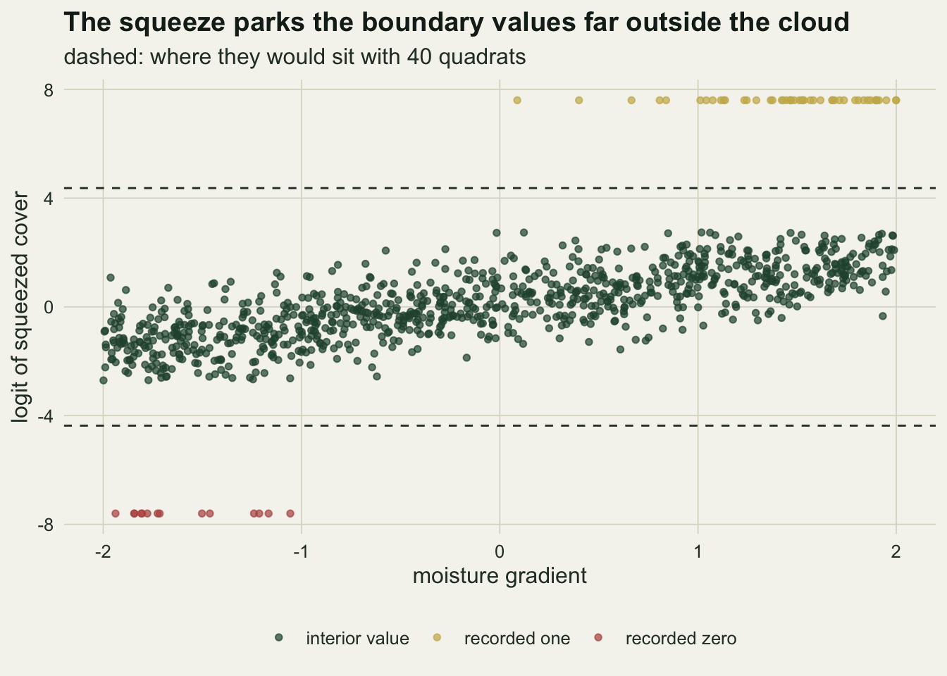
The slope follows the sample size
Beta regression is fitted here by maximum likelihood with optim(), using the analytic score of the mean and precision parameterisation of Ferrari and Cribari-Neto 2004. The standard error comes from the numerical Hessian at the optimum.
nll_beta <- function(par, x, y) {
  mu <- plogis(par[1] + par[2] * x); phi <- exp(par[3])
  -sum(dbeta(y, mu * phi, (1 - mu) * phi, log = TRUE))
}
score_beta <- function(par, x, y) {
  mu <- plogis(par[1] + par[2] * x); phi <- exp(par[3])
  a_sh <- mu * phi; b_sh <- phi - a_sh
  y_star <- qlogis(y); mu_star <- digamma(a_sh) - digamma(b_sh)
  d_eta <- phi * (y_star - mu_star) * mu * (1 - mu)
  d_lphi <- (mu * (y_star - mu_star) + log1p(-y) - digamma(b_sh) + digamma(phi)) * phi
  -c(sum(d_eta), sum(d_eta * x), sum(d_lphi))
}
fit_beta <- function(x, y, se = TRUE) {
  opt <- optim(c(0, 0, 1), nll_beta, score_beta, x = x, y = y, method = "BFGS")
  if (!se) return(c(opt$par, NA))
  hess <- optimHess(opt$par, nll_beta, score_beta, x = x, y = y)
  c(opt$par, sqrt(solve(hess)[2, 2]))
}
Four estimators are compared on every simulated survey. The first fits the latent cover, which no field worker ever sees; it is the control, because any small sample bias of the beta maximum likelihood estimator shows up there without any boundary effect mixed in. The second squeezes the recorded values. The third drops the rows on the boundary. The fourth is the censored beta of the next section, which is included here so that all four see the same data. A fifth fit, not drawn in the figures, applies the squeeze to the latent cover itself: that data set has no zeros or ones, so whatever the squeeze does to it comes from the interior values alone.
nll_cens <- function(par, x, y, floor_val) {
  mu <- plogis(par[1] + par[2] * x); phi <- exp(min(par[3], 8))
  a_sh <- mu * phi; b_sh <- phi - a_sh
  at0 <- y == 0; at1 <- y == 1; inside <- !(at0 | at1)
  -(sum(dbeta(y[inside], a_sh[inside], b_sh[inside], log = TRUE)) +
    sum(pbeta(floor_val, a_sh[at0], b_sh[at0], log.p = TRUE)) +
    sum(pbeta(1 - floor_val, a_sh[at1], b_sh[at1], lower.tail = FALSE, log.p = TRUE)))
}
fit_cens <- function(x, y, floor_val, start, se = TRUE) {
  opt <- optim(start, nll_cens, x = x, y = y, floor_val = floor_val, method = "BFGS")
  if (!se) return(c(opt$par, NA))
  hess <- optimHess(opt$par, nll_cens, x = x, y = y, floor_val = floor_val)
  c(opt$par, sqrt(solve(hess)[2, 2]))
}

one_survey <- function(n, floor_val) {
  d <- make_cover(n, floor_val)
  inside <- d$recorded > 0 & d$recorded < 1
  lat <- fit_beta(d$moist, d$latent)
  sqz <- fit_beta(d$moist, squeeze(d$recorded))
  drp <- fit_beta(d$moist[inside], d$recorded[inside])
  cen <- fit_cens(d$moist, d$recorded, floor_val, start = drp[1:3])
  lsq <- fit_beta(d$moist, squeeze(d$latent), se = FALSE)
  c(share = mean(!inside), est = c(lat[2], sqz[2], drp[2], cen[2]),
    se = c(lat[4], sqz[4], drp[4], cen[4]), lat_sq = lsq[2])
}
The sample size grid runs from 40 to 2500 quadrats. Replicates fall with sample size, because the large fits are slow and also far less variable; the Monte Carlo standard errors below are computed per cell.
n_grid <- c(40, 100, 250, 1000, 2500)
n_reps <- c(300, 200, 150, 100, 60)
est_lev <- c("latent cover (control)", "squeeze", "drop boundary rows", "censored beta")
set.seed(4417)
sim_rows <- list()
for (fl in floors) for (k in seq_along(n_grid)) {
  reps <- replicate(n_reps[k], one_survey(n_grid[k], fl))
  est <- reps[2:5, ]; se <- reps[6:9, ]
  diff_sq <- est[2, ] - est[1, ]
  diff_lsq <- reps[10, ] - est[1, ]
  sim_rows[[length(sim_rows) + 1]] <- data.frame(
    floor_val = fl, n = n_grid[k], reps = n_reps[k], share = mean(reps[1, ]),
    estimator = est_lev, slope = rowMeans(est),
    mcse = apply(est, 1, sd) / sqrt(n_reps[k]),
    cover = rowMeans(abs(est - b1_true) < qnorm(0.975) * se),
    diff_sq = mean(diff_sq), diff_mcse = sd(diff_sq) / sqrt(n_reps[k]),
    diff_lsq = mean(diff_lsq), diff_lsq_mcse = sd(diff_lsq) / sqrt(n_reps[k]))
}
sim_floor <- do.call(rbind, sim_rows)
sim_floor$estimator <- factor(sim_floor$estimator, levels = est_lev)
cell <- function(fl, n, k, what = "slope")
  sim_floor[sim_floor$floor_val == fl & sim_floor$n == n & sim_floor$estimator == est_lev[k], what]
share_lo <- mean(sim_floor$share[sim_floor$floor_val == floors[1]])
share_hi <- mean(sim_floor$share[sim_floor$floor_val == floors[2]])
lat_range <- range(sim_floor$slope[sim_floor$estimator == est_lev[1]])
max_mcse <- max(sim_floor$mcse)
With the lower floor, 1.5 per cent of recorded values are exact zeros or ones. The squeezed slope is 0.778 at 40 quadrats, 0.806 at 250, 0.824 at 1000 and 0.828 at 2500, against a true slope of 0.8. With the higher floor, 6.6 per cent on the boundary, it goes from 0.819 to 0.878, 0.922 and 0.938. The largest Monte Carlo standard error of any mean slope in the grid is 0.007.
The control rules out the obvious alternative explanation. Across every cell the latent fit returns a mean slope between 0.798 and 0.807, so the beta maximum likelihood estimator has little small sample bias at this precision. Because the latent and the squeezed fits use the same survey, the paired difference isolates what the squeeze adds. With the higher floor that difference is 0.012 (Monte Carlo standard error 0.001) at 40 quadrats and 0.138 (0.001) at 2500; with the lower floor it is -0.027 (0.001) at 40 and 0.031 (0.001) at 2500. With the lower floor the squeezed slope is too flat in small surveys and too steep in large ones, so there is a sample size at which it happens to be right, and nothing in the data says which one that is.
With the lower floor the flattening in small surveys has nothing to do with the zeros. Squeezing the latent cover, which has none, moves the slope by -0.032 (0.0006) at 40 quadrats and by -0.002 (0.00003) at 1000: the factor (n - 1)/n pulls every value towards one half, and that pull only matters when n is small. At 40 quadrats it is a larger shift than the squeeze of the recorded data produces, so there the boundary values push the other way, by 0.006. With the higher floor the latent squeeze moves the slope by -0.032 at 40 quadrats and the boundary values add 0.045 on top, enough to reverse the sign. As the survey grows the shrinkage vanishes and the boundary values take over.
Dropping the boundary rows does not depend on sample size in the same way, but it is wrong at every size: 0.775 to 0.766 with the lower floor and 0.704 to 0.699 with the higher. Removing the lowest values at the dry end and the highest at the wet end truncates the response at both ends of the gradient, and the slope flattens.
sim_floor$floor_lab <- factor(sprintf("floor %.2f", sim_floor$floor_val))
ggplot(sim_floor, aes(n, slope, colour = estimator)) +
  geom_hline(yintercept = b1_true, colour = te_body, linetype = "dashed", linewidth = 0.5) +
  geom_errorbar(aes(ymin = slope - 2 * mcse, ymax = slope + 2 * mcse),
                width = 0.08, linewidth = 0.4) +
  geom_line(data = sim_floor[sim_floor$estimator != est_lev[1], ],
            aes(linetype = estimator), linewidth = 0.9) + geom_point(size = 2) +
  geom_line(data = sim_floor[sim_floor$estimator == est_lev[1], ],
            aes(linetype = estimator), linewidth = 1.4) +
  scale_x_log10(breaks = n_grid) +
  scale_colour_manual(values = setNames(c(te_ink, te_rust, te_gold, te_forest), est_lev),
                      limits = est_lev, name = NULL) +
  scale_linetype_manual(values = setNames(c("dotted", "solid", "solid", "solid"), est_lev),
                        limits = est_lev, name = NULL) +
  facet_wrap(~ floor_lab) +
  guides(colour = guide_legend(nrow = 2), linetype = guide_legend(nrow = 2)) +
  labs(x = "quadrats (log scale)", y = "mean fitted slope",
       title = "The squeezed slope depends on how many quadrats there are",
       subtitle = "dashed: the true slope; dotted: the fit to the latent cover") +
  theme_datasheet() + theme(legend.position = "bottom")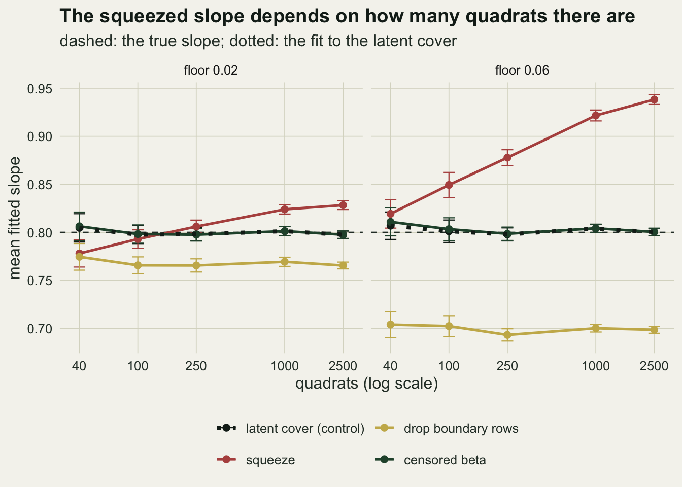
At large n the lever is how far one half divided by n sits from the cloud, not the sample size as such. Replacing the squeeze by a fixed nudge, a zero written as some small number and a one as one minus it, removes the dependence on the number of rows but hands it to the nudge.
nudges <- c(0.05, 0.01, 0.001, 0.0001)
set.seed(5120)
nudge_fit <- replicate(100, {
  d <- make_cover(250, floors[2])
  vapply(nudges, function(e)
    fit_beta(d$moist, pmin(pmax(d$recorded, e), 1 - e), se = FALSE)[2], 0)
})
nudge_slope <- rowMeans(nudge_fit)
For 100 surveys of 250 quadrats with the higher floor, a nudge of 0.05 (just below the floor, so no real value is touched) gives a mean slope of 0.779, a nudge of 0.01 gives 0.838, 0.001 gives 0.904 and 0.0001 gives 0.960. Any of these can be defended in a methods section, and between them they cover every answer from too flat to too steep.
The interval stops covering the truth
A bias that grows while the standard error shrinks has a predictable consequence for the interval.
cov_sq_1000 <- cell(0.06, 1000, 2, "cover"); cov_ce_1000 <- cell(0.06, 1000, 4, "cover")
cov_dr_1000 <- cell(0.06, 1000, 3, "cover"); cov_sq_1000_lo <- cell(0.02, 1000, 2, "cover")
cov_sq_2500_lo <- cell(0.02, 2500, 2, "cover")
cov_mcse_100 <- sqrt(0.95 * 0.05 / 100)
ce_cov_range <- range(sim_floor$cover[sim_floor$estimator == est_lev[4]])
With the higher floor and 1000 quadrats, the nominal 95 per cent Wald interval from the squeezed fit contains the true slope in 1 per cent of surveys, the interval from the dropped rows in 0 per cent, and the censored interval in 95 per cent; with 100 replicates a correct interval would scatter around 95 with a Monte Carlo standard error of 2.2 points. With the lower floor the squeezed interval covers in 83 per cent of surveys at 1000 quadrats and 52 per cent at 2500. Across the whole grid the censored interval covers between 89 and 98 per cent.
ggplot(sim_floor[sim_floor$estimator != est_lev[1], ], aes(n, cover, colour = estimator)) +
  geom_hline(yintercept = 0.95, colour = te_body, linetype = "dashed", linewidth = 0.5) +
  geom_line(linewidth = 0.9) + geom_point(size = 2) +
  scale_x_log10(breaks = n_grid) +
  scale_y_continuous(limits = c(0, 1)) +
  scale_colour_manual(values = c(te_rust, te_gold, te_forest), name = NULL) +
  facet_wrap(~ floor_lab) +
  labs(x = "quadrats (log scale)", y = "interval coverage",
       title = "More quadrats, less coverage",
       subtitle = "the squeeze and the dropped rows lose the truth as the interval narrows") +
  theme_datasheet() + theme(legend.position = "bottom")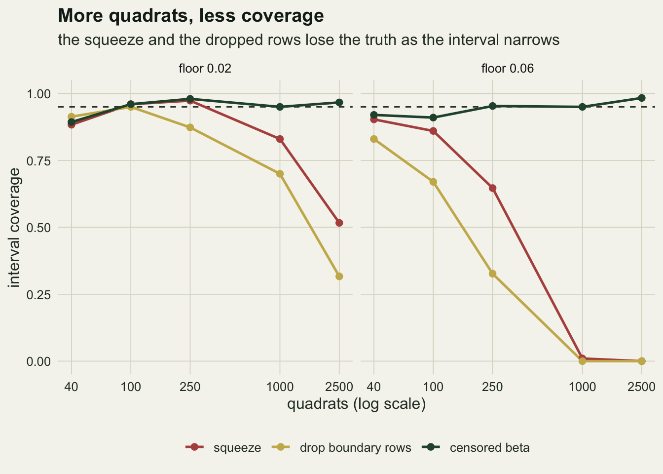
A recording floor is a censored observation
A quadrat written as zero because its cover was below the floor carries the information that the latent cover was somewhere between zero and the floor. Its contribution to the likelihood is therefore the beta distribution function at the floor, pbeta(floor, a, b), and a quadrat written as one contributes the upper tail above one minus the floor. Interior values contribute the beta density as usual. That is nll_cens() above, and it is the same argument the detection limit post makes for a lognormal, applied at both ends of the unit interval.
The simulation has already scored it. The censored slope is 0.811 at 40 quadrats and 0.800 at 2500 with the higher floor, and 0.806 and 0.798 with the lower, tracking the latent control in every cell. It needs one thing the squeeze does not: the value of the floor. Here it was known because it was simulated. In the field it is the smallest cover the protocol lets an observer write, or the class boundary of the cover scale, and it has to be written into the protocol rather than guessed afterwards.
When the zeros are real
The other way to get exact zeros and ones is that they are real. A quadrat with no crowberry in it has cover zero whatever the observer does, and a quadrat inside a closed mat has cover one. That is a different process: some quadrats are boundary quadrats, with a probability of their own, and the rest have a continuous beta cover. The zero-and-one-inflated beta distribution of Ospina and Ferrari 2010 writes exactly this mixture, with a probability of being on the boundary, a conditional probability that a boundary value is a one, and a beta density for everything else; Ospina and Ferrari 2012 develop the regression models for the case with inflation at one end, with covariates on every part, and the version with both ends used here is built the same way.
bnd_logit <- -2.5; one_slope <- 1.5
make_mass <- function(n) {
  moist <- runif(n, -2, 2)
  mu <- plogis(b0_true + b1_true * moist)
  y <- rbeta(n, mu * phi_true, (1 - mu) * phi_true)
  on_bnd <- runif(n) < plogis(bnd_logit)
  y[on_bnd] <- as.numeric(runif(sum(on_bnd)) < plogis(one_slope * moist[on_bnd]))
  list(moist = moist, recorded = y)
}

nll_zoib <- function(par, x, y) {
  on_bnd <- y == 0 | y == 1
  eta_a <- par[1] + par[2] * x; eta_g <- par[3] + par[4] * x
  mu <- plogis(par[5] + par[6] * x); phi <- exp(par[7])
  ll_a <- ifelse(on_bnd, plogis(eta_a, log.p = TRUE), plogis(-eta_a, log.p = TRUE))
  ll_g <- ifelse(y == 1, plogis(eta_g, log.p = TRUE), plogis(-eta_g, log.p = TRUE))
  ll_b <- dbeta(ifelse(on_bnd, 0.5, y), mu * phi, (1 - mu) * phi, log = TRUE)
  -sum(ll_a + on_bnd * ll_g + (!on_bnd) * ll_b)
}

set.seed(6031)
pm <- make_mass(n_large)
pm_in <- pm$recorded > 0 & pm$recorded < 1
zoib <- optim(c(0, 0, 0, 0, 0, 0, 1), nll_zoib, x = pm$moist, y = pm$recorded,
              method = "BFGS", control = list(maxit = 500))
drop_pm <- fit_beta(pm$moist[pm_in], pm$recorded[pm_in], se = FALSE)
zoib_gap <- abs(zoib$par[6] - drop_pm[2])
The joint likelihood splits into three separate pieces: a logistic regression for being on the boundary, a logistic regression for one against zero among the boundary values, and a beta regression on the interior values alone. So the beta part of the inflated model is exactly the drop-the-boundary-rows fit. On one survey of 1000 quadrats, the joint fit by optim() over all seven parameters gives a beta slope of 0.7713 and the interior-only beta fit gives 0.7713, a difference of 1.68e-07 that is optimiser tolerance. The estimator that was biased under a recording floor is the correct one under point masses, because here the interior values are an unselected sample from the beta part.
mass_reps <- c(150, 100, 75, 50, 30)
set.seed(7213)
mass_rows <- lapply(seq_along(n_grid), function(k) {
  n <- n_grid[k]
  reps <- replicate(mass_reps[k], {
    d <- make_mass(n); inside <- d$recorded > 0 & d$recorded < 1
    drp <- fit_beta(d$moist[inside], d$recorded[inside], se = FALSE)
    c(mean(!inside), fit_beta(d$moist, squeeze(d$recorded), se = FALSE)[2], drp[2],
      fit_cens(d$moist, d$recorded, floors[1], start = drp[1:3], se = FALSE)[2])
  })
  data.frame(n = n, share = mean(reps[1, ]),
             estimator = c("squeeze", "inflated beta (beta part)", "censored beta, floor 0.02"),
             slope = rowMeans(reps[2:4, ]), mcse = apply(reps[2:4, ], 1, sd) / sqrt(mass_reps[k]))
})
sim_mass <- do.call(rbind, mass_rows)
sim_mass$estimator <- factor(sim_mass$estimator, levels = unique(sim_mass$estimator))
mcell <- function(n, k) sim_mass$slope[sim_mass$n == n & as.integer(sim_mass$estimator) == k]
mass_share <- mean(sim_mass$share)
With point masses making up 7.9 per cent of the values, the squeezed slope is 0.750 at 40 quadrats and 0.726 at 2500. The beta part of the inflated model gives 0.809 and 0.801. The censored beta, told that the floor was 0.02 when no floor exists, gives 0.788 and 0.779.
ggplot(sim_mass, aes(n, slope, colour = estimator)) +
  geom_hline(yintercept = b1_true, colour = te_body, linetype = "dashed", linewidth = 0.5) +
  geom_errorbar(aes(ymin = slope - 2 * mcse, ymax = slope + 2 * mcse),
                width = 0.08, linewidth = 0.4) +
  geom_line(linewidth = 0.9) + geom_point(size = 2) +
  scale_x_log10(breaks = n_grid) +
  scale_colour_manual(values = c(te_rust, te_forest, te_gold), name = NULL) +
  guides(colour = guide_legend(nrow = 2)) +
  labs(x = "quadrats (log scale)", y = "mean fitted slope",
       title = "Real zeros and ones: the inflated model's beta part is right",
       subtitle = "the squeeze sits below the truth at every size") +
  theme_datasheet() + theme(legend.position = "bottom")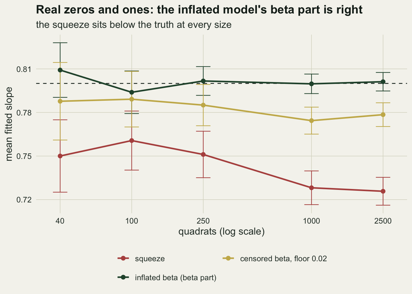
Two models answer two questions
It would be unfair to score the inflated model by its beta slope under a recording floor and stop there. It never claimed to estimate the latent cover. Its target is the recorded cover: how often a quadrat is written as zero or one, and what the rest look like. So the fair comparison asks each model for two curves along the gradient, the expected recorded cover and the expected latent cover, and scores both against the truth.
For the censored beta the expected recorded cover has a closed form. A recorded one contributes the upper tail probability, and the interior contributes the mean times a difference of two beta distribution functions with the first shape raised by one, because y * dbeta(y, a, b) is mu * dbeta(y, a + 1, b).
The discrete part of the inflated model needs one adjustment to be fair. Under a recording floor the chance of a boundary value is high at both ends of the gradient and low in the middle, and a single logistic curve for “on the boundary” can only rise or fall. So the discrete part is written as two logistic regressions, one for a zero against everything else and one for a one against the interior values. It is the same three-part mixture with a different split of the boundary probability, and the beta part is unchanged.
recorded_mean <- function(mu, phi, floor_val) {
  a_sh <- mu * phi; b_sh <- phi - a_sh
  pbeta(1 - floor_val, a_sh, b_sh, lower.tail = FALSE) +
    mu * (pbeta(1 - floor_val, a_sh + 1, b_sh) - pbeta(floor_val, a_sh + 1, b_sh))
}
x_grid <- seq(-2, 2, length.out = 41)
mu_grid <- plogis(b0_true + b1_true * x_grid)
rec_true <- recorded_mean(mu_grid, phi_true, floors[2])

est_reps <- 40
set.seed(8305)
err <- replicate(est_reps, {
  d <- make_cover(n_large, floors[2]); y <- d$recorded; x <- d$moist
  inside <- y > 0 & y < 1; on_bnd <- !inside
  drp <- fit_beta(x[inside], y[inside], se = FALSE)
  zero_fit <- glm(y == 0 ~ x, family = binomial)
  one_fit <- glm(y[y > 0] == 1 ~ x[y > 0], family = binomial)
  p0_g <- plogis(coef(zero_fit)[1] + coef(zero_fit)[2] * x_grid)
  p1_g <- plogis(coef(one_fit)[1] + coef(one_fit)[2] * x_grid)
  mu_zoib <- plogis(drp[1] + drp[2] * x_grid)
  cen <- fit_cens(x, y, floors[2], start = drp[1:3], se = FALSE)
  mu_cen <- plogis(cen[1] + cen[2] * x_grid)
  sqz <- fit_beta(x, squeeze(y), se = FALSE)
  mu_sqz <- plogis(sqz[1] + sqz[2] * x_grid)
  c(zoib_rec = max(abs((1 - p0_g) * (p1_g + (1 - p1_g) * mu_zoib) - rec_true)),
    cen_rec = max(abs(recorded_mean(mu_cen, exp(cen[3]), floors[2]) - rec_true)),
    sqz_rec = max(abs(mu_sqz - rec_true)),
    zoib_lat = max(abs(mu_zoib - mu_grid)),
    cen_lat = max(abs(mu_cen - mu_grid)),
    sqz_lat = max(abs(mu_sqz - mu_grid)))
})
err_mean <- rowMeans(err)
err_mcse_max <- max(apply(err, 1, sd) / sqrt(est_reps))
Over 40 surveys of 1000 quadrats with the higher floor, the largest error along the gradient in the expected recorded cover averages 0.028 for the inflated model, 0.008 for the censored beta and 0.032 for the squeeze. For the expected latent cover the same errors are 0.034 for the inflated model’s beta part, 0.007 for the censored beta and 0.036 for the squeeze, all on the cover scale from zero to one, with Monte Carlo standard errors no larger than 0.0012.
The inflated model does not win on its own target either. That is not a failure of the idea but of its shapes under this mechanism: the interior values behind a floor follow a beta cut off at both ends, which an ordinary beta density does not describe, and the chance of a recorded zero along the gradient follows the lower tail of a beta distribution, not a logistic curve. Its error on the recorded cover is still a few percentage points of cover at worst, which is small for most vegetation work. The model that knows how the zeros were made gets both curves right at once, because the recorded cover is a function of the latent one.
err_df <- data.frame(
  model = factor(rep(c("inflated beta", "censored beta", "squeeze"), 2),
                 levels = c("inflated beta", "censored beta", "squeeze")),
  target = factor(rep(c("recorded cover", "latent cover"), each = 3),
                  levels = c("recorded cover", "latent cover")),
  error = unname(err_mean))
ggplot(err_df, aes(target, error, fill = model)) +
  geom_col(position = position_dodge(width = 0.75), width = 0.65, colour = te_paper, linewidth = 0.3) +
  scale_fill_manual(values = c(te_gold, te_forest, te_rust), name = NULL) +
  labs(x = NULL, y = "largest error along the gradient",
       title = "Under a floor, the censored model gets both curves",
       subtitle = "recording floor 0.06, 1000 quadrats") +
  theme_datasheet() + theme(legend.position = "bottom")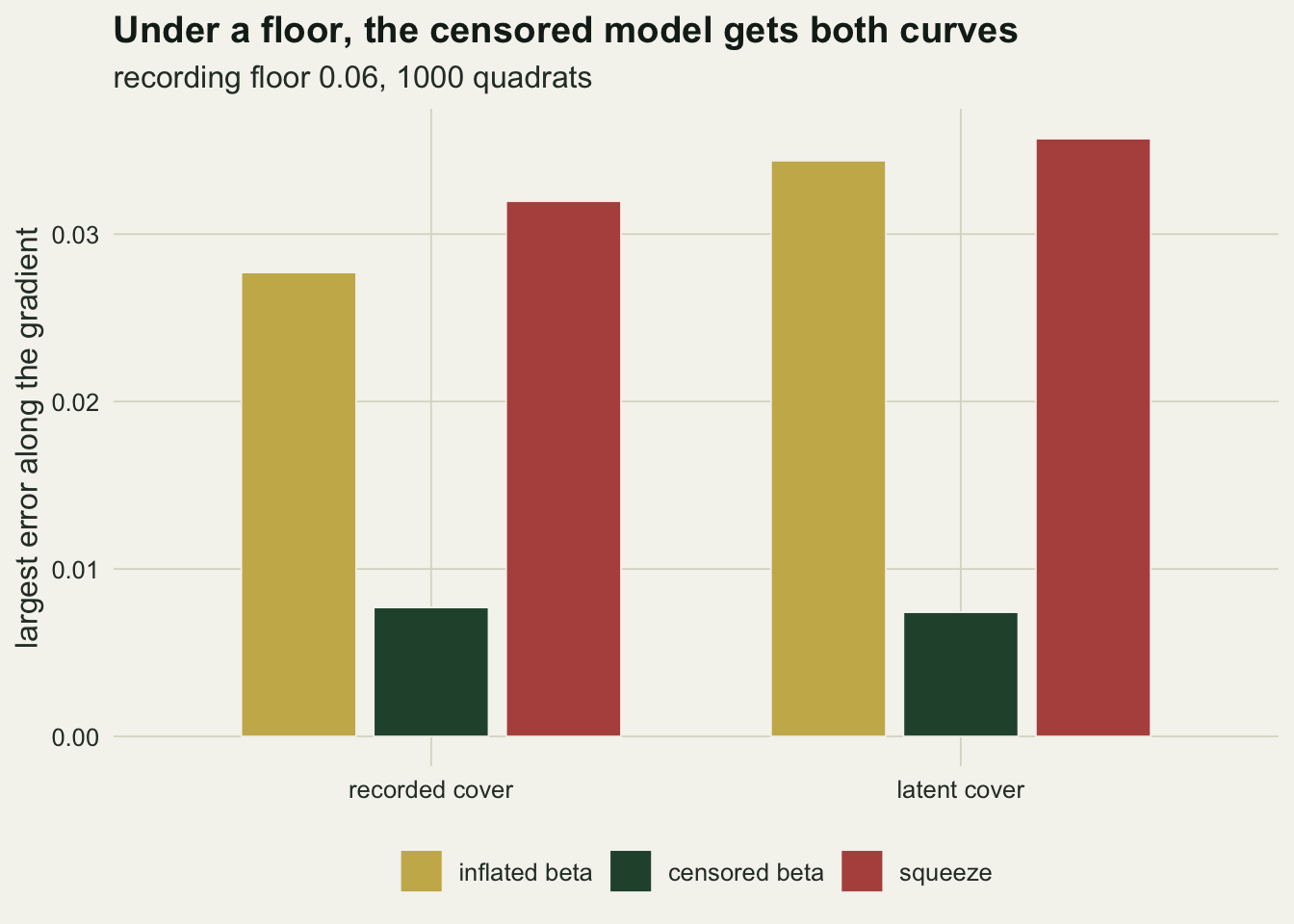
What to report
Say how many values are exact zeros and exact ones, separately, and at which end of the gradient they sit. That count and its position decide how much any of the choices below can matter.
Say what produced them. If the protocol has a smallest cover that can be written, or a cover class whose lower bound is not zero, the zeros are a recording floor and the censored likelihood is the model; report the floor value it was given. If absence and closure are real states of the quadrat, fit the inflated model and report its three parts, because the probability of a zero along the gradient is then an ecological result in its own right.
If the squeeze is used anyway, report the sample size next to the slope and say that the estimate depends on it. Two studies with the same plant and the same gradient but different numbers of quadrats will not agree, and a meta-analysis will read the disagreement as biology. The same applies to a fixed nudge, with the nudge in place of the sample size.
Do not drop the boundary rows without saying so. Under a recording floor that is the estimator with the lowest coverage, or tied for it, in every design of 250 quadrats or more measured here.
Honest limits
The process has a constant precision and a single covariate spread evenly along the gradient. The size of the squeeze effect depends on where the boundary values fall relative to the fitted line, so a design with boundary values in the middle of the gradient, or a precision that changes along it, will give different numbers, possibly of the opposite sign; the point-mass simulation already moves the squeezed slope in the other direction. What carries over is that the answer depends on the sample size, not by how much.
The two mechanisms are pure. In a real survey some zeros are true absences and some are shoots too sparse to record, and a model for that needs both a point mass and a censored part, with the split between them weakly identified unless the protocol records trace presence. Neither the censored nor the inflated model here handles the mixture.
The censored beta was given the true floor. A floor that varies between observers, or a cover scale read by eye to the nearest five per cent, turns the one-sided censoring into interval censoring of every value, which is the case treated in the post on rounded and coarsened measurements and is not simulated here.
The intervals are Wald intervals from a numerical Hessian, and the replicate counts at 1000 and 2500 quadrats are 100 and 60, so coverage near 95 per cent there has a Monte Carlo standard error of 2.2 and 2.8 percentage points. That is enough to separate an interval near 95 per cent from one near zero, and not enough to rank two intervals that both sit near 95.
No package fit was used. The betareg package would return the same slope for the same squeezed data, because the likelihood is the same; the point of fitting by hand is that the censored and inflated likelihoods are then a few lines away from it.
References
Smithson M, Verkuilen J 2006 Psychological Methods 11(1):54-71 (10.1037/1082-989X.11.1.54)
Ferrari SLP, Cribari-Neto F 2004 Journal of Applied Statistics 31(7):799-815 (10.1080/0266476042000214501)
Ospina R, Ferrari SLP 2010 Statistical Papers 51(1):111-126 (10.1007/s00362-008-0125-4)
Ospina R, Ferrari SLP 2012 Computational Statistics and Data Analysis 56(6):1609-1623 (10.1016/j.csda.2011.10.005)