library(ggplot2)
library(patchwork)

te_paper  <- "#f5f4ee"
te_ink    <- "#16241d"
te_body   <- "#2c3a31"
te_forest <- "#275139"
te_rust   <- "#b5534e"
te_gold   <- "#c9b458"
te_line   <- "#dad9ca"

theme_datasheet <- function() {
  theme_minimal(base_size = 12) +
    theme(plot.background  = element_rect(fill = te_paper, colour = NA),
          panel.background = element_rect(fill = te_paper, colour = NA),
          panel.grid.major = element_line(colour = te_line, linewidth = 0.3),
          panel.grid.minor = element_blank(),
          text             = element_text(colour = te_body),
          plot.title       = element_text(colour = te_ink, face = "bold"),
          plot.subtitle    = element_text(colour = te_body),
          axis.text        = element_text(colour = te_body))
}Year lists: cut at the recorder, not the site
R
occupancy
imperfect detection
citizen science
simulation
ecology tutorial
A year list logs a species once per recorder, so the occupancy bias changes sign with sites per recorder. In R: why the site-level removal cut fails, and a fix.
A county dragonfly group asks its members to send in every species they see. Some do exactly that. Others keep a year list: the first banded demoiselle of the season goes in, with date and pond, and after that the species is ticked and never written down again that year, however many ponds it turns up at. Bowler and colleagues asked German recorders how they decide what to report and found the same habit in general form: most would not record the same species twice on the same day in the same place, and they became more likely to report it again the longer it had been since they last saw it. When the season’s records are turned into detection histories for an occupancy model, a year-lister’s visits after that first record look like visits that found nothing.
The post on revisits triggered by sightings names this case among its honest limits and leaves it: year-listing, “where observers log a species only at their first sighting of the year, which is a removal design in disguise. Both deserve their own measurement.” The phrase suggests its own repair. A removal design, in the words of the same post, is one “in which a site stops being visited after its first detection”, and MacKenzie and Royle 2005 give its likelihood; so keep each site’s history up to its first report, drop the rest, and fit that. This post measures the damage and that repair, and finds that the repair works only in the one arrangement where a recorder works a single site. A year list belongs to the recorder, not to the site. Once a lister covers several sites, the forced zeros fall at sites where the lister has not reported yet, whole occupied sites go dark, and beyond a few sites per recorder the naive bias turns downward. Cutting at each site’s first report then makes it worse in all but one of the multi-site cells measured here. The cut that works everywhere is at each recorder’s first report of the year.
Neither the removal likelihood nor the argument for ignoring a stopping rule is new: the second is Rubin 1976, and the source post uses it for extra visits. The limits that the naive and the site-cut estimates converge to also turn out to be arithmetic, so they are derived below and checked against simulation rather than presented as simulation findings. What the simulation adds is what the arithmetic does not give: how the recorder-level cuts behave with few recorders, and what happens when nobody knows who keeps a year list.
Three neighbours set the boundaries. Trap-specific responses in spatial capture-recapture is the mirror image: there the behavioural response is local, to one trap, and a global term cannot fix it; here the response is global, across all of a recorder’s sites, and a local cut cannot fix it. Occupancy from unstructured records shows that recorders who keep their own patches break the independence of visits through differences in skill; year-listing breaks it through the recorder’s memory. What a detection time is worth treats stopping at the first detection as a design chosen in advance and prices it in standard error; here the stop is chosen by the recorder and hidden in the data, and the question is bias. The likelihood itself is the one built by hand in fitting single-season occupancy models in R.
One recorder, five sites, one list
Every simulated county has 300 sites, a true occupancy of 0.40 and a per-visit detection probability of 0.30. Each site is visited six times in the season, once per occasion, and within an occasion the visits across the county come in random order. Recorders work fixed patches: with m sites per recorder there are 300 / m recorders, and every visit to a site is made by the recorder who owns it. Each recorder is a year-lister with probability q. A complete recorder reports every sighting. A year-lister reports the first sighting of the year, at whichever of their sites it happens, and nothing after it. The grid crosses m of 1, 2, 3, 5, 10 and 30 with q of 0.3 and 0.6, with 200 simulated counties per cell. All of these constants were fixed before anything was run.
n_site   <- 300    # sites per county
psi_true <- 0.40   # true occupancy
p_true   <- 0.30   # per-visit detection probability
n_occ    <- 6      # visits per site, one per occasion
m_grid   <- c(1, 2, 3, 5, 10, 30)   # sites per recorder
q_grid   <- c(0.3, 0.6)             # share of recorders who keep a year list
n_draw   <- 200                     # counties per cell

first_of <- function(group, flag, n) {      # index of the first flagged visit in each group
  f <- rep(Inf, n); v <- which(flag); f[rev(group[v])] <- rev(v); f
}

simulate_season <- function(q, m, n = n_site, psi = psi_true, p = p_true, K = n_occ,
                            leak = 0, het = 0) {
  z <- rbinom(n, 1, psi)
  n_rec <- n / m; home <- rep(seq_len(n_rec), each = m)
  lister <- runif(n_rec) < q
  site <- rep(seq_len(n), K)[order(rep(seq_len(K), each = n), runif(n * K))]  # visits in time order
  rec <- home[site]; v <- seq_along(site)
  p_site <- plogis(qlogis(p) + het * rnorm(n))                  # het > 0: detection varies by site
  seen <- runif(n * K) < p_site[site] * z[site]
  first_seen <- first_of(rec, seen, n_rec)
  reported <- seen & (!lister[rec] | v <= first_seen[rec] | runif(n * K) < leak)
  first_rec  <- first_of(rec, reported, n_rec)                  # recorder's first report
  first_site <- first_of(site, reported, n)                     # site's first report
  n_rep <- tabulate(rec[reported], n_rec)
  keep <- list(naive       = rep(TRUE, n * K),
               site_cut    = v <= first_site[site],
               blanket_cut = v <= first_rec[rec],
               known_cut   = !lister[rec] | v <= first_rec[rec],
               class_cut   = n_rep[rec] != 1 | v <= first_rec[rec])
  yn <- lapply(keep, function(k) cbind(y = tabulate(site[k & reported], n), n = tabulate(site[k], n)))
  list(yn = yn, home = home, n_rep = n_rep, n_rec = n_rec)
}
The argument leak lets a year-lister report a later sighting after all, and het lets detection vary between sites; both stay at zero until the last sections. The five keep vectors are the analyses compared below. The naive analysis uses every visit. The site cut keeps each site’s visits up to its first report, the removal design the source post names. The three recorder cuts keep each recorder’s visits up to that recorder’s first report anywhere: for every recorder (the blanket cut), for the recorders known to keep a year list, or for the recorders classified as listers because they made exactly one report all season.
Each analysis ends in the same MacKenzie et al. 2002 likelihood with a different number of retained visits per site: a site with y detections in n retained visits contributes psi p^y (1 - p)^(n - y), plus 1 - psi when y is zero. Sites with the same y and n contribute identical terms, so the fit runs on the collapsed table.
nll_occ <- function(th, y, n, w) {
  psi <- plogis(th[1]); p <- plogis(th[2])
  -sum(w * log(psi * p^y * (1 - p)^(n - y) + (1 - psi) * (y == 0)))
}
fit_occ <- function(yn) {
  yn <- yn[yn[, "n"] > 0, , drop = FALSE]
  key <- yn[, "y"] * 10L + yn[, "n"]; tb <- tabulate(key + 1L); k <- which(tb > 0) - 1L
  o <- optim(c(0, -1), nll_occ, y = k %/% 10L, n = k %% 10L, w = tb[k + 1L], method = "BFGS")
  plogis(o$par[1])
}
Before any estimate, one patch shows where the forced zeros fall. The same five sites, the same sightings and the same visit order are recorded twice: once by five year-listers who each work one site, and once by a single year-lister who works all five. Which sites are occupied is fixed for the picture (sites 1, 2 and 4); the sightings and the order are drawn.
set.seed(33301)
ex_z <- c(1, 1, 0, 1, 0)
ex <- expand.grid(site = 1:5, occ = 1:n_occ)
ex <- ex[order(ex$occ, runif(nrow(ex))), ]
ex$order <- seq_len(nrow(ex))
ex$seen <- runif(nrow(ex)) < p_true * ex_z[ex$site]
ex_first_site <- first_of(ex$site, ex$seen, 5)
ex$rep_own <- ex$seen & ex$order == ex_first_site[ex$site]    # five listers, one site each
ex$rep_one <- ex$seen & ex$order == min(ex$order[ex$seen])     # one lister, five sites
ex_seen_sites <- length(unique(ex$site[ex$seen]))
ex_dark <- ex_seen_sites - length(unique(ex$site[ex$rep_one]))   # seen, but no report under one lister
ex_n_seen <- sum(ex$seen)
c(sightings = ex_n_seen, sites_with_sighting = ex_seen_sites,
  reported_own = sum(ex$rep_own), reported_one = sum(ex$rep_one))
sightings sites_with_sighting reported_own reported_one
6 3 3 1 ex_state <- function(rep_col) {
s <- ifelse(ex[[rep_col]], "reported",
ifelse(ex$seen, "seen, not listed",
ifelse(ex_z[ex$site] == 1, "occupied, not seen", "empty site")))
factor(s, levels = c("reported", "seen, not listed", "occupied, not seen", "empty site"))
}
ex_long <- rbind(data.frame(ex, state = ex_state("rep_own"), who = "five listers, one site each"),
data.frame(ex, state = ex_state("rep_one"), who = "one lister, five sites"))
ex_long$who <- factor(ex_long$who, levels = c("five listers, one site each", "one lister, five sites"))
ex_long$site_lab <- factor(sprintf("site %d%s", ex_long$site, ifelse(ex_z[ex_long$site] == 1, " (occupied)", "")),
levels = rev(sprintf("site %d%s", 1:5, ifelse(ex_z == 1, " (occupied)", ""))))
ggplot(ex_long, aes(occ, site_lab, fill = state)) +
geom_tile(colour = te_paper, linewidth = 1.2) +
geom_text(aes(label = order, colour = state %in% c("reported", "seen, not listed")), size = 3.1,
show.legend = FALSE) +
facet_wrap(~ who) +
scale_fill_manual(values = c("reported" = te_forest, "seen, not listed" = te_rust,
"occupied, not seen" = te_gold, "empty site" = te_line),
name = NULL, drop = FALSE) +
scale_colour_manual(values = c("FALSE" = te_body, "TRUE" = te_paper)) +
scale_x_continuous(breaks = 1:n_occ) +
labs(x = "occasion", y = NULL, title = "The same sightings, two kinds of year list") +
theme_datasheet() +
theme(legend.position = "bottom", panel.grid.major = element_blank(),
strip.text = element_text(colour = te_ink, face = "bold"))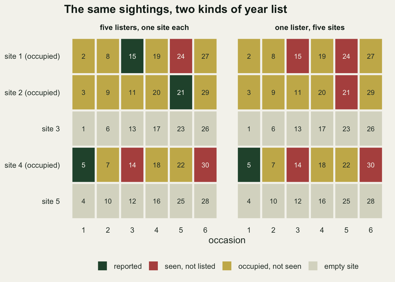
The patch has 6 sightings, at all three of its occupied sites. With one lister per site, every site where the species was seen keeps its first sighting, and the lost sightings sit after a report on the same row: the site looks occupied with poor detection. With one lister for the patch, 1 sighting is reported and the other 5 vanish, and 2 sites where the species was seen have no report at all: they look empty.
The naive fit has a closed form
The naive estimate can be written down without simulation. The occupancy likelihood with every site visited K times is a zero-inflated binomial, and it factorises. Put \(\theta = \psi\{1 - (1-p)^K\}\), the chance that a site produces at least one report under the model. Then
\[ L(\psi, p) = \theta^{\,n_{+}} (1-\theta)^{\,n_{0}} \prod_{i:\,y_i > 0} \frac{\binom{K}{y_i} p^{y_i} (1-p)^{K - y_i}}{1 - (1-p)^K}, \]
where \(n_+\) sites have a report and \(n_0\) have none. The first part gives \(\hat\theta = n_+ / (n_+ + n_0)\), the share of sites with a report. The product is a zero-truncated binomial, an exponential family in \(p\), so \(\hat p\) solves \(Kp / \{1 - (1-p)^K\} = \bar y_+\), the mean number of reports per reported site. Finally \(\hat\psi = \hat\theta / \{1 - (1-\hat p)^K\}\) when that ratio is below one; otherwise the fit sits at the boundary \(\hat\psi = 1\), where \(\hat p\) is simply the number of reports per visit. As the number of recorders grows, \(\hat\theta\) and \(\bar y_+\) tend to their expectations, and those follow from the design.
Write \(w = \psi\{1 - (1-p)^K\}\) for the chance that a site is occupied and the species is seen there at least once. A complete recorder reports all of it: a share \(w\) of their sites carries a report, with \(Kp\psi\) reports per site on average. A year-lister who works \(m\) sites reports once in the year if they see the species anywhere, which happens with probability \(1 - (1 - w)^m\), and that one report sits at one site. Per site worked,
\[ \theta^{*} = (1-q)\,w + q\,\frac{1 - (1-w)^m}{m}, \qquad \bar y_+^{*} = \frac{(1-q)\,K p \psi + q\,\{1 - (1-w)^m\}/m}{\theta^{*}} . \]
With one site per recorder, \(\{1 - (1-w)^m\}/m = w\), so \(\theta^{*}\) is exactly right: every site where the species was seen still has its report. Only \(\bar y_+^{*}\) falls, \(\hat p\) falls with it, and \(\hat\psi\) rises. With several sites per recorder, \(\{1 - (1-w)^m\}/m\) is smaller than \(w\), whole sites drop out of \(\theta^{*}\), and that pulls \(\hat\psi\) down, against the fall in \(\hat p\) that pushes it up. Which force wins depends on \(m\).
The site cut has a closed form of the same kind. Each site keeps its visits up to its first report, which is the removal likelihood: a site first reported at visit \(t\) contributes \(\psi (1-p)^{t-1} p\), a site never reported \(1 - \psi + \psi(1-p)^K\). It factorises in the same way, with \(\hat\theta\) unchanged and \(\hat p\) solving \(\sum_t t\,p(1-p)^{t-1} / \{1 - (1-p)^K\} = \bar t_+\), the mean occasion of the first report among reported sites. At a complete recorder’s site that occasion has the right distribution. A year-lister’s one report comes at the occasion \(T\) of their first sighting anywhere, with \(P(T \le t) = 1 - \{1 - \psi + \psi(1-p)^t\}^m\): the earliest of several sites’ waiting times. With \(m = 1\) that is the right distribution too, which is why the removal cut that the source post’s phrase suggests is exact for one-site recorders. With \(m > 1\) the reports come too early, \(\hat p\) comes out too high, and \(\hat\psi\) comes out too low, on top of the sites that went dark.
solve_p <- function(target, fn) uniroot(function(p) fn(p) - target, c(1e-9, 1 - 1e-9), tol = 1e-12)$root
plim <- function(q, m, psi = psi_true, p = p_true, K = n_occ) {
  w <- psi * (1 - (1 - p)^K)
  r_list <- (1 - (1 - w)^m) / m                        # reported sites per site worked, for a lister
  theta <- (1 - q) * w + q * r_list
  y_plus <- ((1 - q) * psi * K * p + q * r_list) / theta
  p_naive <- if (y_plus <= 1 + 1e-12) 0 else solve_p(y_plus, function(pp) K * pp / (1 - (1 - pp)^K))
  psi_naive <- theta / (1 - (1 - p_naive)^K)
  if (psi_naive >= 1) {                                # no interior fit: occupancy at the boundary of one,
    psi_naive <- 1; p_naive <- theta * y_plus / K      # detection = reports per visit
  }
  tt <- 1:K
  pt_list <- diff(c(0, 1 - (1 - psi + psi * (1 - p)^tt)^m))  # occasion of a lister's first sighting
  t_plus <- ((1 - q) * psi * sum(tt * p * (1 - p)^(tt - 1)) + q / m * sum(tt * pt_list)) / theta
  p_site <- solve_p(t_plus, function(pp) sum(tt * pp * (1 - pp)^(tt - 1)) / (1 - (1 - pp)^K))
  psi_site <- theta / (1 - (1 - p_site)^K)
  if (psi_site >= 1) {                                 # same boundary for the removal likelihood
    psi_site <- 1; p_site <- theta / (theta * t_plus + (1 - theta) * K)
  }
  c(naive = psi_naive, p_naive = p_naive, site = psi_site, p_site = p_site, theta = theta)
}
cf_one <- sapply(c(0.1, 0.3, 0.6, 0.9, 1), function(q) plim(q, 1))
cf_cells <- expand.grid(m = m_grid, q = q_grid)
cf_cells <- cbind(cf_cells, t(mapply(plim, cf_cells$q, cf_cells$m)))

big_n <- 30000                                   # one very large county per cell
set.seed(33302)
cf_cells$big_naive <- NA_real_; cf_cells$big_site <- NA_real_
for (i in seq_len(nrow(cf_cells))) {
  s <- simulate_season(cf_cells$q[i], cf_cells$m[i], n = big_n)
  cf_cells$big_naive[i] <- fit_occ(s$yn$naive); cf_cells$big_site[i] <- fit_occ(s$yn$site_cut)
}
cf_gap <- max(abs(c(cf_cells$big_naive - cf_cells$naive, cf_cells$big_site - cf_cells$site)))
round(cf_cells, 3)
m q naive p_naive site p_site theta big_naive big_site
1 1 0.3 0.449 0.226 0.400 0.300 0.353 0.451 0.404
2 2 0.3 0.417 0.236 0.373 0.314 0.334 0.416 0.374
3 3 0.3 0.393 0.245 0.354 0.324 0.320 0.396 0.355
4 5 0.3 0.361 0.257 0.329 0.334 0.300 0.358 0.325
5 10 0.3 0.324 0.275 0.303 0.336 0.277 0.323 0.303
6 30 0.3 0.295 0.291 0.286 0.318 0.257 0.294 0.285
7 1 0.6 0.588 0.142 0.400 0.300 0.353 0.593 0.405
8 2 0.6 0.495 0.156 0.347 0.330 0.316 0.489 0.343
9 3 0.6 0.428 0.169 0.310 0.353 0.287 0.424 0.310
10 5 0.6 0.344 0.191 0.262 0.383 0.248 0.342 0.262
11 10 0.6 0.255 0.227 0.210 0.401 0.200 0.252 0.210
12 30 0.6 0.190 0.270 0.173 0.357 0.161 0.184 0.167For one site per recorder the limit of the naive estimate is 0.412, 0.449 and 0.588 when a tenth, three tenths and six tenths of the recorders keep a year list, with detection pulled down to 0.276, 0.226 and 0.142 from the true 0.30. At 0.9 the ratio for \(\hat\psi\) exceeds one, so the fit sits at the boundary: occupancy 1.000 and detection 0.065, the reports per visit. When every recorder keeps a year list, each reported site has exactly one report, \(\bar y_+ = 1\), the zero-truncated equation has no root inside (0, 1), and the fit goes to the same boundary: occupancy 1.000 and detection 0.059. The multi-site limits are just as much arithmetic; the simulations below check them and then go where the arithmetic does not.
The check is one county of 30 000 sites per cell of the grid, fitted by the same code as everything else. Across all twelve cells and both analyses, the fitted estimate and the closed form differ by at most 0.006.
The sign follows the number of sites
The main grid runs 200 ordinary counties of 300 sites in each of the twelve cells and fits all the analyses to each. The mixture model in the last column is introduced in a later section.
yn_grid <- expand.grid(y = 0:n_occ, n = 0:n_occ)
n_pat <- nrow(yn_grid)
pattern_counts <- function(yn, home, n_rec) {    # recorders x (y, n) patterns
  pat <- yn[, "y"] + (n_occ + 1L) * yn[, "n"] + 1L
  matrix(tabulate((home - 1L) * n_pat + pat, n_rec * n_pat), n_rec, n_pat, byrow = TRUE)
}
nll_mix <- function(th, d) {
  psi <- plogis(th[1]); p <- plogis(th[2]); q <- plogis(th[3])
  y <- yn_grid$y; n <- yn_grid$n
  ll <- ifelse(n == 0 | y > n, 0, log(psi * p^y * (1 - p)^pmax(n - y, 0) + (1 - psi) * (y == 0)))
  a <- log(q) + as.numeric(d$ct %*% ll); a[d$multi] <- -Inf   # lister: cut at first report
  b <- log1p(-q) + as.numeric(d$cf %*% ll)                     # complete: every visit
  mx <- pmax(a, b)
  -sum(d$w * (mx + log(exp(a - mx) + exp(b - mx))))
}
fit_mix <- function(s) {
  cf <- pattern_counts(s$yn$naive, s$home, s$n_rec)
  ct <- pattern_counts(s$yn$blanket_cut, s$home, s$n_rec)
  multi <- s$n_rep > 1                                          # two reports: cannot be a lister
  key <- apply(cbind(cf, ct, multi), 1, paste, collapse = ",")
  u <- !duplicated(key)
  d <- list(cf = cf[u, , drop = FALSE], ct = ct[u, , drop = FALSE], multi = multi[u],
            w = as.numeric(table(key)[key[u]]))
  best <- NULL
  for (st in list(c(0, -1, -1), c(0, -1, 1))) {                 # two starts for the lister share
    o <- optim(st, nll_mix, d = d, method = "BFGS")
    if (is.null(best) || o$value < best$value) best <- o
  }
  c(psi = plogis(best$par[1]), q = plogis(best$par[3]))
}
one_draw <- function(q, m, ...) {
  s <- simulate_season(q, m, ...)
  mx <- fit_mix(s)
  c(sapply(s$yn, fit_occ), mix = mx[["psi"]], mix_q = mx[["q"]])   # mix_q: estimated share of listers
}
summarise_draws <- function(d, ...) data.frame(..., estimator = colnames(d),
  med = apply(d, 2, median), lo = apply(d, 2, quantile, 0.25), hi = apply(d, 2, quantile, 0.75),
  mean = colMeans(d), sd = apply(d, 2, sd), bnd = colMeans(d > 0.99), row.names = NULL)
cells <- expand.grid(m = m_grid, q = q_grid)
set.seed(33303)
grid_draws <- lapply(seq_len(nrow(cells)), function(i)
t(replicate(n_draw, one_draw(cells$q[i], cells$m[i]))))
summ <- do.call(rbind, lapply(seq_len(nrow(cells)), function(i)
summarise_draws(grid_draws[[i]], m = cells$m[i], q = cells$q[i])))
st <- function(est, m, q, col = "med") summ[[col]][summ$estimator == est & summ$m == m & summ$q == q]
cf_at <- function(m, q, col) cf_cells[[col]][cf_cells$m == m & cf_cells$q == q]
multi_cells <- summ$m > 1
site_rows <- summ[summ$estimator == "site_cut" & multi_cells, ]
site_worse <- abs(site_rows$med - psi_true) > abs(summ$med[summ$estimator == "naive" & multi_cells] - psi_true)
site_exc <- site_rows[!site_worse, c("m", "q")]
known_dev <- max(abs(summ$med[summ$estimator == "known_cut" & multi_cells] - psi_true))
mcse_max <- max(summ$sd[!summ$estimator %in% c("blanket_cut", "mix_q")]) / sqrt(n_draw)
lim_z <- do.call(rbind, lapply(c("naive", "site_cut"), function(e) { # simulation mean against its limit
r <- summ[summ$estimator == e, ]; lim <- mapply(cf_at, r$m, r$q, MoreArgs = list(col = sub("_cut", "", e)))
data.frame(m = r$m, q = r$q, estimator = e, gap = r$mean - lim, z = (r$mean - lim) / (r$sd / sqrt(n_draw)))
}))
lim_gap <- max(abs(lim_z$gap))
round(xtabs(med ~ m + estimator, summ[summ$q == 0.3, ]), 3) estimator
m blanket_cut class_cut known_cut mix mix_q naive site_cut
1 0.400 0.378 0.398 0.398 0.302 0.447 0.400
2 0.402 0.393 0.400 0.399 0.298 0.416 0.374
3 0.389 0.399 0.397 0.397 0.302 0.392 0.350
5 0.409 0.413 0.405 0.405 0.296 0.367 0.335
10 0.511 0.406 0.404 0.403 0.280 0.330 0.311
30 0.508 0.395 0.395 0.395 0.300 0.284 0.281With three recorders in ten keeping a year list, the limit of the naive estimate is 0.449 when each recorder works one site, 0.417 at two sites, 0.393 at three, 0.361 at five, 0.324 at ten and 0.295 at thirty, against a truth of 0.40. With six in ten the limits run from 0.588 to 0.344 at five sites and 0.190 at thirty. More year-listers push both ends further from the truth and move the crossing point out: at three sites per recorder the limit is 0.393 with three listers in ten and 0.428 with six. The simulated counties follow the limits: with three listers in ten the naive median is 0.447 at one site, 0.367 at five and 0.284 at thirty, and over all twelve cells the mean of the naive and of the site-cut estimates is never more than 0.010 from its limit. The largest Monte Carlo standard error of a cell mean in the grid, the blanket cut apart, is 0.0059.
The site cut, the removal design, does what the arithmetic says. At one site per recorder its limit is the truth, and its median is 0.400 and 0.405 for the two shares of listers: it is the right analysis there. At five sites per recorder its limit is 0.329 and 0.262, below the naive 0.361 and 0.344, and at thirty sites 0.286 and 0.173. The detection estimate behind it shows the mechanism: in the five-site cell with three listers in ten its limit is 0.334, above the true 0.30, while the naive fit’s is 0.257. The naive fit kept the zeros after each lister’s single report, and those zeros were holding detection down and occupancy up, partly offsetting the dark sites. Cutting at the site’s first report removes exactly those zeros and leaves the dark sites. In 9 of the 10 multi-site cells the site cut ends further from the truth than doing nothing; the exception is 2 sites per recorder with 6 listers in ten, where the naive estimate is 0.498 and the site cut 0.348.
cf_line <- do.call(rbind, lapply(q_grid, function(qq) {
  mm <- 1:30; v <- sapply(mm, function(m) plim(qq, m))
  rbind(data.frame(m = mm, q = qq, analysis = "naive, every visit", psi = v["naive", ]),
        data.frame(m = mm, q = qq, analysis = "cut at the site's first report", psi = v["site", ]))
}))
grid_pts <- summ[summ$estimator %in% c("naive", "site_cut"), ]
grid_pts$analysis <- ifelse(grid_pts$estimator == "naive", "naive, every visit", "cut at the site's first report")
lvl <- c("naive, every visit", "cut at the site's first report")
cf_line$analysis <- factor(cf_line$analysis, levels = lvl); grid_pts$analysis <- factor(grid_pts$analysis, levels = lvl)
q_lab <- function(x) sprintf("%s in 10 recorders keep a year list", c("0.3" = "3", "0.6" = "6")[as.character(x)])
cf_line$qf <- factor(q_lab(cf_line$q)); grid_pts$qf <- factor(q_lab(grid_pts$q))
p_grid <- ggplot(grid_pts, aes(m, mean, colour = analysis)) +
  geom_hline(yintercept = psi_true, colour = te_ink, linetype = "dashed", linewidth = 0.6) +
  geom_line(data = cf_line, aes(m, psi), linewidth = 0.9) +
  geom_errorbar(aes(ymin = mean - 2 * sd / sqrt(n_draw), ymax = mean + 2 * sd / sqrt(n_draw)),
                width = 0.06, linewidth = 0.5) +
  geom_point(size = 2.4) +
  facet_wrap(~ qf) +
  scale_colour_manual(values = c(te_gold, te_rust), name = NULL) +
  scale_x_log10(breaks = m_grid) +
  labs(x = "sites per recorder (log scale)", y = "estimated occupancy",
       title = "The year list turns the bias round",
       subtitle = "dashed line: true occupancy 0.40") +
  theme_datasheet() +
  theme(legend.position = "bottom", strip.text = element_text(colour = te_ink, face = "bold"))
p_grid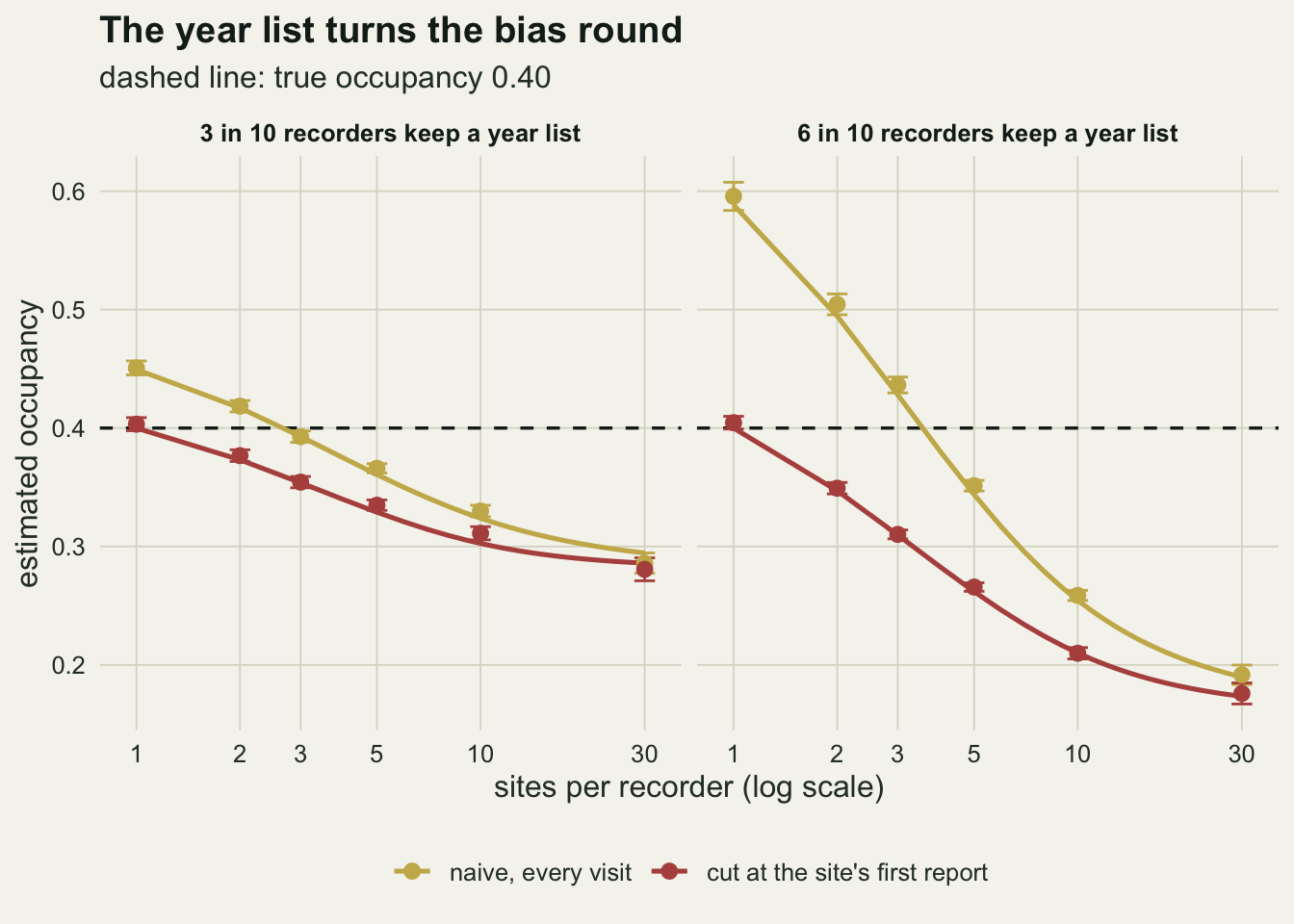
Cut at the recorder, not the site
A year list is a stopping rule at the level of the recorder: after the recorder’s first report of the year, their probability of reporting the species drops to zero at every site they work. The cut that matches it keeps each lister’s visits up to that recorder’s first report, wherever it was made, and drops every visit after it, including visits to sites the lister had not yet reported. For a recorder known to keep a year list this is not a loss of information. Every visit after the cut reports nothing with probability one whether the site is occupied or not, so it multiplies the likelihood by one; the likelihood of the retained visits is the full likelihood of the model in which a lister’s detection probability falls to zero after the first report. It is the occupancy version of a behavioural-response model with the post-response detection fixed at zero, and the retained visits obey Rubin’s condition because the cut reads only what was recorded.
known_med <- summ$med[summ$estimator == "known_cut"]
blanket_sd_30 <- st("blanket_cut", 30, 0.3, "sd"); known_sd_30 <- st("known_cut", 30, 0.3, "sd")
blanket_bnd <- max(summ$bnd[summ$estimator == "blanket_cut"])
naive_sd_1 <- st("naive", 1, 0.3, "sd"); known_sd_1 <- st("known_cut", 1, 0.3, "sd")
round(xtabs(med ~ m + estimator, summ[summ$q == 0.6, ]), 3)
estimator
m blanket_cut class_cut known_cut mix mix_q naive site_cut
1 0.405 0.388 0.404 0.405 0.596 0.589 0.405
2 0.405 0.395 0.404 0.404 0.601 0.498 0.348
3 0.398 0.402 0.404 0.403 0.611 0.430 0.309
5 0.409 0.407 0.402 0.404 0.602 0.346 0.263
10 0.568 0.404 0.402 0.401 0.603 0.256 0.209
30 0.512 0.400 0.400 0.400 0.600 0.186 0.169The known-lister cut has a median between 0.395 and 0.405 across all twelve cells; in the multi-site cells it is never further than 0.005 from 0.40. Its spread between counties is 0.032 at one site per recorder with three listers in ten, against 0.042 for the naive fit, and 0.042 at thirty sites.
Cutting every recorder at their first report, listers or not, needs no knowledge of who keeps a year list, and it is equally valid as a likelihood: it is also a stopping rule on the record. It is also wasteful, because it throws away a complete recorder’s later visits, which did carry information, and it keeps at most one detection per recorder. With five sites per recorder its median is 0.409; with thirty sites the county has ten recorders, the retained data hold at most ten detections, and the estimate falls apart: median 0.508, spread 0.210 against 0.042 for the known-lister cut, and in the worst cell 30 per cent of counties with an estimate at the boundary of one. That is a problem of too little retained information, not of bias in the argument, and it is already visible at five sites per recorder, where the blanket cut’s spread is 0.114 against 0.033.
rec_lab <- c(known_cut = "cut known listers", blanket_cut = "cut every recorder",
             class_cut = "cut one-report recorders", mix = "recorder-type mixture")
rec_pts <- summ[summ$estimator %in% names(rec_lab), ]
rec_pts$analysis <- factor(unname(rec_lab[rec_pts$estimator]), levels = rec_lab)
rec_pts$qf <- factor(q_lab(rec_pts$q))
rec_pts$mf <- factor(rec_pts$m, levels = m_grid)
ggplot(rec_pts, aes(mf, med, colour = analysis, shape = analysis)) +
  geom_hline(yintercept = psi_true, colour = te_ink, linetype = "dashed", linewidth = 0.6) +
  geom_errorbar(aes(ymin = lo, ymax = hi), width = 0, linewidth = 0.7,
                position = position_dodge(width = 0.7)) +
  geom_point(size = 2.4, fill = te_paper, stroke = 1, position = position_dodge(width = 0.7)) +
  facet_wrap(~ qf) +
  scale_colour_manual(values = c(te_forest, te_gold, te_rust, te_ink), name = NULL) +
  scale_shape_manual(values = c(16, 16, 16, 23), name = NULL) +
  guides(colour = guide_legend(nrow = 2), shape = guide_legend(nrow = 2)) +
  labs(x = "sites per recorder", y = "estimated occupancy",
       title = "A cut at the recorder holds; cutting everyone gets noisy",
       subtitle = "dashed line: true occupancy 0.40") +
  theme_datasheet() +
  theme(legend.position = "bottom", strip.text = element_text(colour = te_ink, face = "bold"))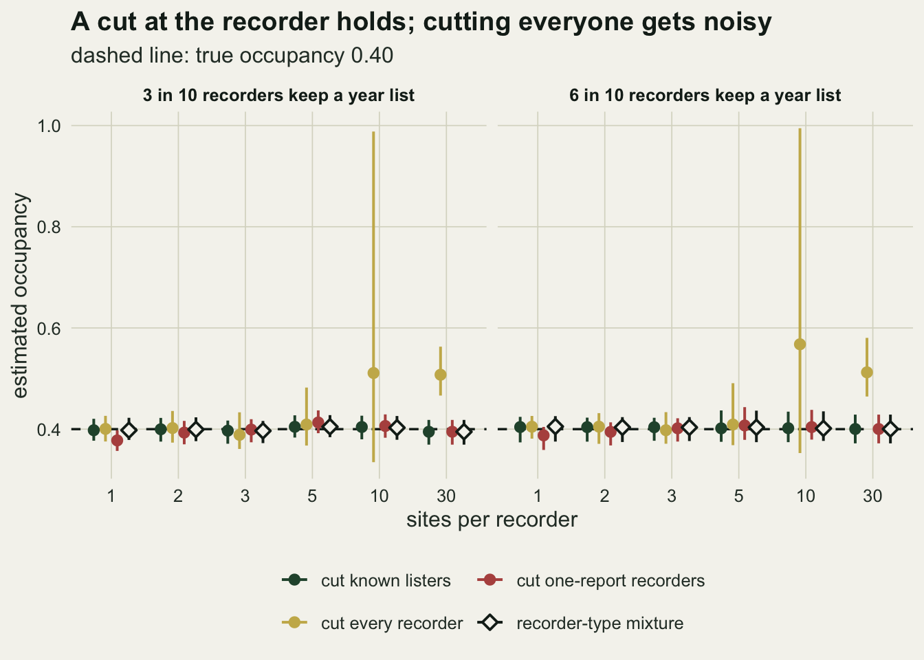
When nobody says who keeps a year list
Recording schemes rarely store whether a member keeps a year list. The obvious proxy is behaviour: a recorder who made exactly one report of the species all season is treated as a lister, and cut at that report. With several sites per recorder the proxy is close to harmless: at five sites its median is 0.413 and 0.407. With one site per recorder it is biased low, 0.378 and 0.388. The reason is that the classification reads the future. A complete recorder whose site produced a single detection is classified as a lister, and the zeros after that detection are dropped, but those were genuine zeros, and whether a second report ever came is decided by the very visits being dropped. That is not a stopping rule, and Rubin’s condition does not cover it. With several sites per recorder a complete recorder rarely ends the season with a single report, so few are misclassified.
A likelihood can do the classification instead. Treat each recorder’s type as unknown, a lister with probability \(q\) to be estimated. Given the type, the recorder’s data factorise over their sites: a lister contributes the retained visits up to their first report, and is impossible if they reported twice; a complete recorder contributes every visit. The recorder’s likelihood is \(q L_{\text{lister}} + (1 - q) L_{\text{complete}}\), and the county’s is the product over recorders. The fit_mix() function above is that model, fitted from two starting values of \(q\). Its median is 0.398 and 0.405 at one site per recorder, and between 0.395 and 0.405 over the whole grid. At one site per recorder it identifies the listers from the shape of the counts and the timing of single reports: listers produce sites with exactly one report more often than a binomial allows, and earlier in the season. That identification rests on the detection model being right, so the chunk below tries it where it is not: detection varying between sites, with a standard deviation of 1 on the logit scale, and a county with no listers at all.
rob_cells <- expand.grid(m = c(1, 5), q = c(0, 0.3), het = c(0, 1))
rob_cells <- rob_cells[!(rob_cells$q == 0.3 & rob_cells$het == 0), ]    # already in the main grid
set.seed(33304)
rob <- do.call(rbind, lapply(seq_len(nrow(rob_cells)), function(i)
  summarise_draws(t(replicate(n_draw, one_draw(rob_cells$q[i], rob_cells$m[i], het = rob_cells$het[i]))),
                  m = rob_cells$m[i], q = rob_cells$q[i], het = rob_cells$het[i])))
rb <- function(est, m, q, het) rob$med[rob$estimator == est & rob$m == m & rob$q == q & rob$het == het]
rob$cell <- sprintf("m %2d, q %.1f, het %d", rob$m, rob$q, rob$het)
mix_known_gap <- max(abs(rob$med[rob$estimator == "mix" & rob$het == 1] - rob$med[rob$estimator == "known_cut" & rob$het == 1]))
mixq <- c(hom = st("mix_q", 1, 0.3), null_1 = rb("mix_q", 1, 0, 1), null_5 = rb("mix_q", 5, 0, 1),
          het_1 = rb("mix_q", 1, 0.3, 1), het_5 = rb("mix_q", 5, 0.3, 1))   # median estimated share of listers
round(mixq, 3)
hom null_1 null_5 het_1 het_5
0.302 0.100 0.017 0.371 0.323 round(xtabs(med ~ cell + estimator, rob), 3) estimator
cell blanket_cut class_cut known_cut mix mix_q naive site_cut
m 1, q 0.0, het 0 0.398 0.375 0.400 0.394 0.005 0.400 0.398
m 1, q 0.0, het 1 0.350 0.333 0.343 0.339 0.100 0.343 0.350
m 1, q 0.3, het 1 0.351 0.337 0.346 0.342 0.371 0.371 0.351
m 5, q 0.0, het 0 0.409 0.416 0.406 0.407 0.002 0.406 0.404
m 5, q 0.0, het 1 0.353 0.348 0.341 0.344 0.017 0.341 0.348
m 5, q 0.3, het 1 0.353 0.350 0.344 0.346 0.323 0.309 0.298With no year-listers and constant detection, the one-report rule still pulls the estimate to 0.375 at one site per recorder, while the naive fit and the mixture give 0.400 and 0.394: the classifier’s bias does not need listers to exist. Detection that varies between sites drags every analysis down, as it always does in occupancy models: with no listers the naive fit gives 0.343 at one site per recorder. With three listers in ten on top of that, the naive fit gives 0.371 at one site and 0.309 at five, the known-lister cut 0.346 and 0.344, and the mixture 0.342 and 0.346. In every heterogeneous cell the mixture lands within 0.005 of the known-lister cut: it removes the year-list part of the bias and leaves the heterogeneity part, which needs its own model.
The estimated share of listers holds up less well than the occupancy estimate. With constant detection it is on target, a median of 0.302 against a true 0.30 at one site per recorder. With site-varying detection and no listers at all, the mixture still puts 0.100 of recorders on the year list at one site per recorder (0.017 at five sites), and with three listers in ten it gives 0.371 at one site and 0.323 at five, against a true 0.30. A lister is the only departure from a single binomial that the mixture can express, so part of the heterogeneity is read as year-listing, most of all when each recorder works one site.
A year list that leaks
Bowler and colleagues found that people become more likely to record a species again as time passes since they last saw it, so a real year list leaks. The next cells let a lister report a later sighting with a fixed probability, 0.2 or 0.5 per sighting after the first, at one and at five sites per recorder with three listers in ten.
leak_cells <- expand.grid(m = c(1, 5), leak = c(0.2, 0.5))
set.seed(33305)
lk <- do.call(rbind, lapply(seq_len(nrow(leak_cells)), function(i)
  summarise_draws(t(replicate(n_draw, one_draw(0.3, leak_cells$m[i], leak = leak_cells$leak[i]))),
                  m = leak_cells$m[i], leak = leak_cells$leak[i])))
lv <- function(est, m, leak) lk$med[lk$estimator == est & lk$m == m & lk$leak == leak]
lk$cell <- sprintf("m %d, leak %.1f", lk$m, lk$leak)
lk_dev5 <- max(abs(lk$med[lk$estimator %in% c("class_cut", "mix") & lk$m == 5] - psi_true))
round(xtabs(med ~ cell + estimator, lk), 3)
estimator
cell blanket_cut class_cut known_cut mix mix_q naive site_cut
m 1, leak 0.2 0.400 0.378 0.397 0.405 0.194 0.434 0.400
m 1, leak 0.5 0.399 0.379 0.399 0.406 0.069 0.417 0.399
m 5, leak 0.2 0.402 0.408 0.396 0.397 0.143 0.376 0.355
m 5, leak 0.5 0.409 0.413 0.396 0.400 0.030 0.396 0.380A leak shrinks the damage. At five sites per recorder the naive median moves from 0.367 with a strict year list to 0.376 and 0.396, so at the stronger leak the naive fit has almost no bias left; the site cut moves from 0.335 to 0.355 and 0.380, and stays low. The known-lister cut is untouched by the leak, 0.396 and 0.396, because whatever a lister does after the cut is not in the data it keeps. A leaking lister who reports twice is treated as a complete recorder by the one-report rule and by the mixture, so the sightings that lister still withheld stay in the data as zeros; at five sites per recorder both methods nevertheless stay within 0.013 of the truth at either leak.
Where the crossover sits
The sign of the naive bias depends on the number of sites per recorder, and the point where it changes depends on detection. The closed form gives it at no cost. The figure repeats the two limits for detection probabilities of 0.15, 0.30 and 0.50, with three listers in ten.
p_cf <- c(0.15, 0.3, 0.5); m_cf <- 1:30
cross_tab <- expand.grid(p = p_cf, q = c(0.15, 0.3, 0.6))
cross_tab$m_star <- mapply(function(pp, qq) {
  nv <- sapply(m_cf, function(m) plim(qq, m, p = pp)[["naive"]]); min(m_cf[nv < psi_true])
}, cross_tab$p, cross_tab$q)
site_max <- max(sapply(p_cf, function(pp) sapply(c(0.15, 0.3, 0.6), function(qq)
  max(sapply(2:30, function(m) plim(qq, m, p = pp)[["site"]])))))
cross_tab
p q m_star
1 0.15 0.15 5
2 0.30 0.15 3
3 0.50 0.15 2
4 0.15 0.30 6
5 0.30 0.30 3
6 0.50 0.30 2
7 0.15 0.60 7
8 0.30 0.60 4
9 0.50 0.60 3cr_line <- do.call(rbind, lapply(p_cf, function(pp) {
v <- sapply(m_cf, function(m) plim(0.3, m, p = pp))
rbind(data.frame(m = m_cf, p = pp, analysis = "naive, every visit", psi = v["naive", ]),
data.frame(m = m_cf, p = pp, analysis = "cut at the site's first report", psi = v["site", ]))
}))
cr_line$analysis <- factor(cr_line$analysis, levels = lvl)
cr_line$pf <- factor(sprintf("detection %.2f", cr_line$p))
ggplot(cr_line, aes(m, psi, colour = pf)) +
geom_hline(yintercept = psi_true, colour = te_ink, linetype = "dashed", linewidth = 0.6) +
geom_line(linewidth = 0.9) +
facet_wrap(~ analysis) +
scale_colour_manual(values = c(te_rust, te_gold, te_forest), name = NULL) +
scale_x_log10(breaks = m_grid) +
labs(x = "sites per recorder (log scale)", y = "limit of the occupancy estimate",
title = "Low detection moves the crossover, not the site cut",
subtitle = "three in ten recorders keep a year list; dashed line: truth") +
theme_datasheet() +
theme(legend.position = "bottom", strip.text = element_text(colour = te_ink, face = "bold"))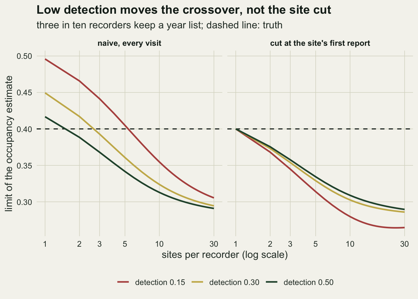
With three listers in ten, the naive estimate first falls below the truth at 6 sites per recorder when detection is 0.15, at 3 when it is 0.30 and at 2 when it is 0.50; with six in ten the three values are 7, 4 and 3. So the crossover is not a fixed patch size, and a given data set can sit on either side of it. The site cut does not have that ambiguity: over these three detection probabilities, three shares of listers and every patch size from two to thirty, its limit is never above 0.388. Whenever year-listers work more than one site, the removal cut is biased low.
What to report
Say how records reach the data set before any estimate: whether recorders submit complete lists, whether some log a species once a year, and how many sites a typical recorder covers. The last number, together with detection, decides the sign of the naive bias. With three listers in ten and detection 0.30, the limit of the naive estimate is 0.449 against a true 0.40 when each recorder works one site and 0.361 at five sites.
Do not treat year-listed data as a removal design at the site. Cutting each site’s history at its first report is right only when every recorder works a single site; at five sites per recorder its limit is 0.329, further from the truth than the uncorrected fit’s.
Where the scheme records who submitted each record, cut each recorder known to keep a year list at their first report of the species, wherever it was made, and drop their later visits at every site. That is the full likelihood for those recorders, not a discarded sample. Cutting every recorder the same way is valid but wasteful, and with few recorders it becomes unstable.
Where lister status is unknown and recorders cover several sites, treating one-report recorders as listers came within 0.013 of the truth in the multi-site cells. Where each recorder covers a single site, that rule is biased even when nobody keeps a year list; the recorder-type mixture is the alternative, and its answer should be reported next to the naive one. Its estimated share of listers is inflated when detection varies between sites, so on its own it is not evidence that anyone keeps a year list.
Honest limits
A visit here is one recorder at one site on one occasion. Real schemes reconstruct visits as lists by date, site and recorder, and a list can pool several people, some of whom keep year lists and some not. Whether a cut at the recorder can be applied to such a pooled visit, or whether the pooled visit needs its own detection model, was not measured. Nor was the arrangement in which recorders roam across the county and many recorders visit each site; there a lister’s forced zeros spread thinly over many sites and the patch-size argument does not apply directly.
The leak is a constant probability of re-reporting, applied to every later sighting. The behaviour Bowler and colleagues describe is a probability that rises with time since the last observation, so a real lister is closer to a year list in spring and closer to a complete recorder by autumn; the constant leak shows that the direction survives and the size shrinks, not how a time-varying leak behaves.
Everything is a single season with constant occupancy, and detection is constant except in the heterogeneity cells, where the mixture was tried but no heterogeneity model was fitted. Every site gets six visits, one per occasion, all by its own recorder; the closed forms rest on that balanced design, and uneven visit numbers would change the limits, though not the argument for where to cut. Year-listing across years, and the false trend it could create as recording habits change, is a separate problem that this post does not touch.
The main grid uses 200 counties per cell, and the heterogeneity and leak cells use the same number. Leaving out the blanket cut, whose spread is in a class of its own, the Monte Carlo standard error of a cell mean is at most 0.0059, so differences between analyses smaller than about two of those are not resolved. The closed forms were checked against one county of 30 000 sites per cell rather than against many.
References
MacKenzie DI, Nichols JD, Lachman GB, Droege S, Royle JA, Langtimm CA 2002 Ecology 83(8):2248-2255 (10.1890/0012-9658(2002)083[2248:ESORWD]2.0.CO;2)
MacKenzie DI, Royle JA 2005 Journal of Applied Ecology 42(6):1105-1114 (10.1111/j.1365-2664.2005.01098.x)
Rubin DB 1976 Biometrika 63(3):581-592 (10.1093/biomet/63.3.581)
Bowler DE, Bhandari N, Repke L, Beuthner C, Callaghan CT, Eichenberg D, Henle K, Klenke R, Richter A, Jansen F, Bruelheide H, Bonn A 2022 Scientific Reports 12:11069 (10.1038/s41598-022-15218-2)