library(ggplot2)

te_paper  <- "#f5f4ee"
te_ink    <- "#16241d"
te_body   <- "#2c3a31"
te_forest <- "#275139"
te_rust   <- "#b5534e"
te_gold   <- "#c9b458"
te_line   <- "#dad9ca"

theme_datasheet <- function() {
  theme_minimal(base_size = 12) +
    theme(plot.background  = element_rect(fill = te_paper, colour = NA),
          panel.background = element_rect(fill = te_paper, colour = NA),
          panel.grid.major = element_line(colour = te_line, linewidth = 0.3),
          panel.grid.minor = element_blank(),
          text             = element_text(colour = te_body),
          plot.title       = element_text(colour = te_ink, face = "bold"),
          plot.subtitle    = element_text(colour = te_body),
          axis.text        = element_text(colour = te_body))
}Spatial cross-validation when the target is a map
R
cross-validation
spatial statistics
kriging
model validation
ecology tutorial
Block or random cross-validation for a kriged map? Simulated in R: block folds overstate a random sample’s map error, random folds understate a clustered one.
A county ecologist has 150 grassland plots, each with a measured standing biomass, and two covariates that exist for every cell of the county: a greenness index and a soil wetness index. She fits biomass on the two covariates, kriges the residuals, and publishes a map. The report needs a number for how wrong the map is. Random ten-fold cross-validation gives one number; a reviewer, pointing at a variogram with obvious structure, asks for spatial block cross-validation, and that gives a number about half as large again. Both are defensible on paper. Only one of them is the error of the map she is publishing.
This post is about that choice, and the answer does not come from the residuals. It comes from where the sample sits relative to the cells being mapped. Spatial cross-validation for SDMs blocks because held-out points next to training points flatter a model on new ground, and it measures that optimistic direction; its closing section adds, in one sentence of prose, that random folds “may match the intended use” when the goal is to interpolate inside a well-surveyed region. Checking a tree ensemble turns the blocking argument into a rule, “Report a blocked error, not the out-of-bag number, whenever location carries information”, measured on uniformly random points with no true error to say which of its two numbers was right. When the thing published is a map of the region that was sampled at random, the same rule overstates the map’s error and can erase most of a real spatial term, and the check that settles which scheme to use is a comparison of two distance distributions, made before any fold is drawn.
The idea that a validation scheme estimates a particular quantity, and that the wrong scheme estimates a different one, is already on the site. Data leakage in ecological model validation says it for grouped rows: random folds “estimate a different one: the error of predicting a new visit to a site you have already characterised”. What this post adds is spatial distance in place of group membership, an exact map error as the truth, a sample-design arm that reverses the direction of the bias, and a diagnostic that is run on the coordinates alone. Kriging itself is introduced in from scattered plots to a surface, which scores ordinary kriging with plain leave-one-out and has no design arm.
None of the headline results are new. Wadoux, Heuvelink, de Bruin and Brus found in a 2021 biomass mapping experiment that spatial cross-validation was a more biased estimate of map accuracy than the standard kind, and argued that with a probability sample the design-based estimate of map accuracy is unbiased, so no spatial correction is needed (the design-based machinery is in design-based variance and spatial balance). Ploton and colleagues showed the opposite failure on a large forest biomass map of Africa, where a non-spatial validation suggested the model explained more than half the variation and a spatial one found almost none. Mila, Mateu, Pebesma and Meyer proposed nearest neighbour distance matching (NNDM) leave-one-out to sit between the two. This post is a demonstration of those papers on a map small enough to know the true error of every cell. What is measured here is narrower: how the block overshoot depends on the block side and on the residual range together, how far each scheme misstates the gain from the kriging term in both directions, whether the distance comparison picks the right scheme before any fold is drawn, and how much NNDM scatters when a clustered sample has only fifteen clusters.
A map, two samples and the number being estimated
The map is the unit square cut into a 64 by 64 grid of cells. Each of the two covariates is white noise smoothed by a Gaussian kernel (standard deviations 0.10 and 0.20 of the map side), standardised over the map. The residual field is built the same way with kernel standard deviation s, and the response in every cell is the first covariate plus half the second plus the residual field; a plot measurement adds independent noise with standard deviation 0.4, which plays the role of the nugget. Three residual scales are run, s = 0.03, 0.06 and 0.12.
Two samples of 150 plots are drawn from the cells. The random design is a simple random sample. The clustered design is fifteen clusters of ten plots each, every cluster drawn from the cells within 0.06 of a centre placed uniformly in the central part of the map, which is roughly what a survey looks like when plots follow road access or a handful of cooperating landowners.
The model is ordinary least squares on the two covariates followed by simple kriging of its residuals. The kriging uses the covariance of the process that generates the residual field, so the only error the cross-validation has to judge is the error of estimation, not the error of a fitted variogram; a later section refits the kernel from the data to see whether that matters. The same model without the kriging step, least squares alone, is carried along as the comparison for the gain.
g_side  <- 64
g_torus <- 128
cell_x  <- (rep(seq_len(g_side), times = g_side) - 0.5) / g_side
cell_y  <- (rep(seq_len(g_side), each = g_side) - 0.5) / g_side
xy_all  <- cbind(cell_x, cell_y)
n_cell  <- g_side^2
nug_sd  <- 0.4
n_samp  <- 150
n_clus  <- 15
clus_r  <- 0.06

# Gaussian-kernel smoothed white noise on a torus, cropped and standardised
smooth_field <- function(s_ker) {
  noise <- matrix(rnorm(g_torus * g_torus), g_torus)
  lag_d   <- pmin(0:(g_torus - 1), g_torus - 0:(g_torus - 1)) / g_side
  kern  <- outer(exp(-lag_d^2 / (2 * s_ker^2)), exp(-lag_d^2 / (2 * s_ker^2)))
  fld   <- Re(fft(fft(noise) * fft(kern), inverse = TRUE))[1:g_side, 1:g_side]
  v <- as.vector(fld)
  (v - mean(v)) / sd(v)
}
cross_dist <- function(a, b) {
  sqrt(outer(a[, 1], b[, 1], "-")^2 + outer(a[, 2], b[, 2], "-")^2)
}
# white noise smoothed by a Gaussian kernel of sd s has covariance exp(-d^2 / (4 s^2))
cov_fun <- function(d, s_ker, sill = 1) sill * exp(-d^2 / (4 * s_ker^2))

draw_sample <- function(design) {
  if (design == "random") return(sample(n_cell, n_samp))
  cen <- cbind(runif(n_clus, 0.08, 0.92), runif(n_clus, 0.08, 0.92))
  idx <- integer(0)
  for (k in seq_len(n_clus)) {
    d_cen <- sqrt((cell_x - cen[k, 1])^2 + (cell_y - cen[k, 2])^2)
    cand  <- setdiff(which(d_cen < clus_r), idx)
    idx   <- c(idx, cand[sample.int(length(cand), n_samp / n_clus)])
  }
  idx
}
# least squares on the two covariates, then simple kriging of the residuals
fit_pred <- function(itr, new_xy, new_x, s_ker, y, xmat, xy, dmat,
krige = TRUE, sill = 1, nug = nug_sd^2) {
des <- cbind(1, xmat[itr, , drop = FALSE])
coef_ls <- qr.solve(des, y[itr])
resid_tr <- y[itr] - des %*% coef_ls
mu <- cbind(1, new_x) %*% coef_ls
if (!krige) return(as.vector(mu))
kmat <- cov_fun(dmat[itr, itr], s_ker, sill)
diag(kmat) <- diag(kmat) + nug
k0 <- cov_fun(cross_dist(new_xy, xy[itr, , drop = FALSE]), s_ker, sill)
as.vector(mu + k0 %*% solve(kmat, resid_tr))
}
cv_rmse <- function(folds, s_ker, y, xmat, xy, dmat, krige = TRUE,
sill = 1, nug = nug_sd^2) {
pr <- numeric(length(y))
for (f in folds) {
pr[f$te] <- fit_pred(f$tr, xy[f$te, , drop = FALSE], xmat[f$te, , drop = FALSE],
s_ker, y, xmat, xy, dmat, krige, sill, nug)
}
sqrt(mean((pr - y)^2))
}The number every scheme is trying to estimate is fixed before any fold is drawn. The model is fitted to all 150 plots and predicts every cell that holds no plot, 3946 of them. The true map error is the root mean squared difference between those predictions and the true cell values, with the nugget variance added so that it sits on the same footing as a cross-validated error, which is scored against noisy plot measurements. It is the error of this map over this region: not over a new region, and not over the sample.
s_vals   <- c(0.03, 0.06, 0.12)
range_05 <- 2 * s_vals * sqrt(log(20))
names(range_05) <- s_vals
cor_side <- exp(-0.2^2 / (4 * s_vals^2))
# each field is centred and rescaled over the map: realised correlation at a lag of 13 cells
set.seed(128)
lag_c <- 13
real_cor <- mean(replicate(40, {
  zm <- matrix(smooth_field(0.12), g_side)
  (mean(zm[1:(g_side - lag_c), ] * zm[(1 + lag_c):g_side, ]) +
     mean(zm[, 1:(g_side - lag_c)] * zm[, (1 + lag_c):g_side])) / 2
}))
proc_cor <- exp(-(lag_c / g_side)^2 / (4 * 0.12^2))
A block side means something only against the range of the residual field, so the range has to be defined before any side is quoted. Here it is the distance at which the residual correlation, exp(-d^2 / (4 s^2)) for a Gaussian kernel of standard deviation s applied to white noise, falls to 0.05; that distance is 2 s sqrt(ln 20), which gives 0.104, 0.208 and 0.415 for the three scales. A block of side 0.2 is therefore close to one range at s = 0.06, about two ranges at s = 0.03 and about half a range at s = 0.12, where two cells 0.2 apart still have a residual correlation of 0.50 in the process. Each simulated field is then centred and rescaled over the map, which lowers the correlation a single map actually shows: at a lag of 13 cells (0.203) and s = 0.12 it averages 0.37 over 40 fields, against 0.49 for the process. The kriging uses the process covariance, so at the longest scale it assumes more correlation than the fields it is applied to actually show.
random_folds <- function(n, n_fold = 10) {
  fr <- sample(rep(seq_len(n_fold), length.out = n))
  lapply(seq_len(n_fold), function(k) list(te = which(fr == k), tr = which(fr != k)))
}
# square blocks of side 1 / k_side, blocks dealt at random to five folds
block_folds <- function(xy, k_side, n_fold = 5) {
  bid <- as.integer(factor(paste(ceiling(xy[, 1] * k_side), ceiling(xy[, 2] * k_side))))
  bf  <- sample(rep(seq_len(n_fold), length.out = max(bid)))[bid]
  lapply(seq_len(n_fold), function(k) list(te = which(bf == k), tr = which(bf != k)))
}
# NNDM leave-one-out: a line-by-line port of the loop in CAST::nndm (Mila et al. 2022)
nndm_folds <- function(dmat, gpred, min_train = 0.5) {
  n <- nrow(dmat)
  tdist <- dmat
  diag(tdist) <- NA
  phi   <- max(c(gpred, c(tdist)), na.rm = TRUE) + 1e-9
  gstar <- apply(tdist, 1, min, na.rm = TRUE)
  rmin  <- min(gstar)
  jmin  <- which.min(gstar)[1]
  kmin  <- which(tdist[jmin, ] == rmin)
  while (rmin <= phi) {
    if ((sum(gstar <= rmin) - 1) / n >= mean(gpred <= rmin) &&
        sum(!is.na(tdist[jmin, ])) / n > min_train) {
      tdist[jmin, kmin] <- NA
      gstar[jmin] <- min(tdist[jmin, ], na.rm = TRUE)
      rmin <- min(gstar[gstar >= rmin])
    } else if (sum(gstar > rmin) == 0) {
      break
    } else {
      rmin <- min(gstar[gstar > rmin])
    }
    jmin <- which(gstar == rmin)[1]
    kmin <- which(tdist[jmin, ] == rmin)
  }
  lapply(seq_len(n), function(j) list(te = j, tr = which(!is.na(tdist[j, ]))))
}
# distance from each held-out point to the nearest point its fold trains on
test_nn <- function(folds, dmat) {
  te_all <- unlist(lapply(folds, `[[`, "te"))
  nn_all <- unlist(lapply(folds, function(f) apply(dmat[f$te, f$tr, drop = FALSE], 1, min)))
  nn_all[order(te_all)]
}
# area between two empirical distribution functions (the W statistic of Mila et al.)
w_stat <- function(a, b) {
  gr <- sort(unique(c(a, b)))
  sum(abs(ecdf(a)(gr) - ecdf(b)(gr))[-length(gr)] * diff(gr))
}
Three families of scheme are compared. Random ten-fold deals the plots to folds at random. Block five-fold cuts the map into squares of side 0.1, 0.2 or 1/3 and deals whole squares to five folds, which is what a block cross-validation package does with a regular grid. NNDM leave-one-out holds out one plot at a time, and before it predicts that plot it also removes from the training set every plot closer than it needs to be: the removals continue, smallest distance first, until the distribution of held-out-to-training distances matches the distribution of distances from the prediction cells to the sample. The function above is a line-by-line port of the loop in the CAST package’s nndm(), with its defaults (no training set shrinks below half the data, and the search runs to the largest distance in the data). Plain leave-one-out is not run and carries no number below.
The last two helpers are the diagnostic. test_nn() returns, for each plot, the distance to the nearest plot its fold trains on; w_stat() is the area between two empirical distribution functions, the statistic Mila and colleagues use to say how far a scheme’s distances are from the prediction distances. Neither needs a response value or a model fit.
set.seed(61)
z_show  <- smooth_field(0.06)
idx_ran <- draw_sample("random")
idx_clu <- draw_sample("clustered")
lab_ran <- "simple random sample"
lab_clu <- "15 clusters of 10"
field_df <- rbind(data.frame(x = cell_x, y = cell_y, z = z_show, design = lab_ran),
                  data.frame(x = cell_x, y = cell_y, z = z_show, design = lab_clu))
plot_df  <- rbind(data.frame(x = cell_x[idx_ran], y = cell_y[idx_ran], design = lab_ran),
                  data.frame(x = cell_x[idx_clu], y = cell_y[idx_clu], design = lab_clu))
ggplot(field_df, aes(x, y)) +
  geom_raster(aes(fill = z)) +
  geom_hline(yintercept = seq(0.2, 0.8, by = 0.2), colour = te_ink, linewidth = 0.25, alpha = 0.6) +
  geom_vline(xintercept = seq(0.2, 0.8, by = 0.2), colour = te_ink, linewidth = 0.25, alpha = 0.6) +
  geom_point(data = plot_df, shape = 21, size = 1.6, fill = te_ink, colour = te_paper, stroke = 0.4) +
  facet_wrap(~ factor(design, levels = c(lab_ran, lab_clu))) +
  scale_fill_gradient2(low = te_forest, mid = te_paper, high = te_rust, midpoint = 0,
                       name = "residual\nfield") +
  coord_equal(expand = FALSE) +
  labs(x = NULL, y = NULL, title = "The same map, two ways of sampling it",
       subtitle = "residual kernel sd 0.06; thin dark lines: blocks of side 0.2") +
  theme_datasheet() +
  theme(axis.text = element_blank(), panel.grid.major = element_blank())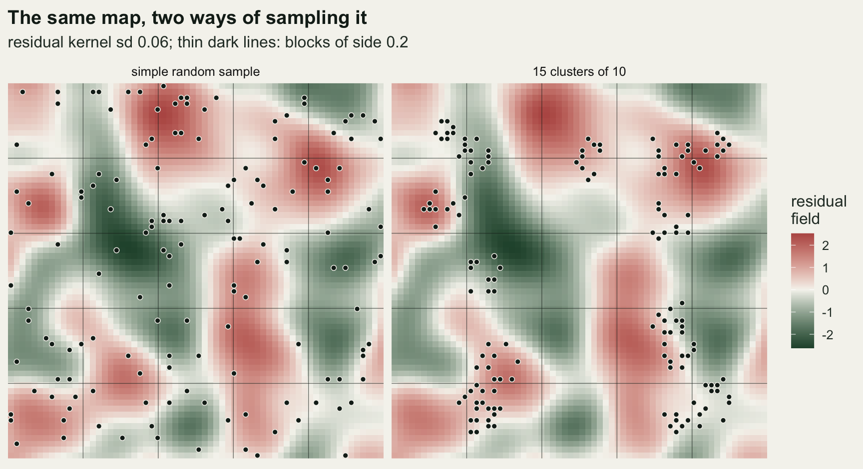
Five schemes against the true map error
Each draw makes new covariates, a new residual field and a new sample, fits the model once to the whole sample for the truth, and runs every scheme on the same draw, with and without the kriging step. The replication was fixed before the run: 40 draws per design at s = 0.06, the headline scale, and 20 per design at the other two scales. At s = 0.06 on the random design the draw also runs a sweep of seven block sides, and at s = 0.06 on both designs it refits the kernel, for the sections further down.
fit_kernel <- function(dmat, resid_all) {
  s_grid   <- exp(seq(log(0.01), log(0.3), length.out = 25))
  tau_grid <- c(0.02, 0.05, 0.1, 0.2, 0.4, 0.8)
  loglik <- outer(s_grid, tau_grid, Vectorize(function(sg, tg) {
    vm <- exp(-dmat^2 / (4 * sg^2))
    diag(vm) <- 1 + tg
    ch <- chol(vm)
    u  <- backsolve(ch, resid_all, transpose = TRUE)
    -0.5 * (length(u) * log(sum(u^2) / length(u)) + 2 * sum(log(diag(ch))))
  }))
  best <- which(loglik == max(loglik), arr.ind = TRUE)[1, ]
  s_hat <- s_grid[best[1]]
  tau_hat <- tau_grid[best[2]]
  vm <- exp(-dmat^2 / (4 * s_hat^2))
  diag(vm) <- 1 + tau_hat
  sill_hat <- sum(resid_all * solve(vm, resid_all)) / length(resid_all)
  c(s = s_hat, sill = sill_hat, nug = sill_hat * tau_hat)
}

one_draw <- function(s_ker, design, k_sides = c(10, 5, 3), fitted = FALSE) {
  x1 <- smooth_field(0.10)
  x2 <- smooth_field(0.20)
  z  <- smooth_field(s_ker)
  mu_all <- x1 + 0.5 * x2 + z
  x_all  <- cbind(x1, x2)
  idx  <- draw_sample(design)
  y    <- mu_all[idx] + rnorm(n_samp, 0, nug_sd)
  xmat <- x_all[idx, ]
  xy   <- xy_all[idx, ]
  pc   <- setdiff(seq_len(n_cell), idx)
  dmat <- as.matrix(dist(xy))
  gpred <- apply(cross_dist(xy_all[pc, ], xy), 1, min)
  folds <- c(list(rand10 = random_folds(n_samp)),
             setNames(lapply(k_sides, function(k) block_folds(xy, k)),
                      paste0("blk", k_sides)),
             list(nndm = nndm_folds(dmat, gpred)))
  w_vals <- sapply(folds, function(f) w_stat(test_nn(f, dmat), gpred))
  out <- c()
  for (kr in c(TRUE, FALSE)) {
    pred  <- fit_pred(seq_len(n_samp), xy_all[pc, ], x_all[pc, ], s_ker,
                      y, xmat, xy, dmat, kr)
    truth <- sqrt(mean((pred - mu_all[pc])^2) + nug_sd^2)
    cvs   <- sapply(folds, cv_rmse, s_ker = s_ker, y = y, xmat = xmat,
                    xy = xy, dmat = dmat, krige = kr)
    out <- c(out, setNames(c(truth, cvs),
                           paste0(if (kr) "rk_" else "lm_", c("truth", names(folds)))))
  }
  out <- c(out, setNames(w_vals, paste0("W_", names(w_vals))))
  if (fitted) {
    kp <- fit_kernel(dmat, lm.fit(cbind(1, xmat), y)$residuals)
    pred  <- fit_pred(seq_len(n_samp), xy_all[pc, ], x_all[pc, ], kp["s"],
                      y, xmat, xy, dmat, TRUE, kp["sill"], kp["nug"])
    truth <- sqrt(mean((pred - mu_all[pc])^2) + nug_sd^2)
    cvs   <- sapply(folds[c("rand10", "blk5", "nndm")], cv_rmse, s_ker = kp["s"],
                    y = y, xmat = xmat, xy = xy, dmat = dmat, krige = TRUE,
                    sill = kp["sill"], nug = kp["nug"])
    out <- c(out, fit_truth = truth, setNames(cvs, paste0("fit_", names(cvs))),
             s_hat = unname(kp["s"]))
  }
  out
}
s_head <- 0.06
n_head <- 40
n_other <- 20
k_sweep <- c(12, 10, 8, 6, 5, 4, 3)
set.seed(3270)
cells <- list()
for (s_ker in s_vals) for (des in c("random", "clustered")) {
is_head <- s_ker == s_head
ks <- if (is_head && des == "random") k_sweep else c(10, 5, 3)
cells[[paste(s_ker, des)]] <- t(replicate(if (is_head) n_head else n_other,
one_draw(s_ker, des, ks, fitted = is_head)))
}
n_draw_total <- sum(sapply(cells, nrow))
ratio_of <- function(cell, scheme, pre = "rk") {
cells[[cell]][, paste0(pre, "_", scheme)] / cells[[cell]][, paste0(pre, "_truth")]
}
gain_of <- function(cell, scheme) {
m <- cells[[cell]]
(m[, paste0("lm_", scheme)] - m[, paste0("rk_", scheme)]) / (m[, "lm_truth"] - m[, "rk_truth"])
}
fmt_q <- function(v) sprintf("%.2f [%.2f, %.2f]", median(v), min(v), max(v))
fmt_m <- function(v) sprintf("%.2f", median(v))
scheme_lab <- c(rand10 = "random 10-fold", blk10 = "block, side 0.1",
blk5 = "block, side 0.2", blk3 = "block, side 1/3",
nndm = "NNDM leave-one-out")
ratio_tab <- do.call(rbind, lapply(names(cells), function(cl) {
parts <- strsplit(cl, " ")[[1]]
do.call(rbind, lapply(names(scheme_lab), function(sc) {
v <- ratio_of(cl, sc)
data.frame(s_ker = as.numeric(parts[1]), design = parts[2], scheme = sc,
med = median(v), lo = min(v), hi = max(v))
}))
}))q <- function(cl, sc, pre = "rk") fmt_q(ratio_of(cl, sc, pre))
qm <- function(cl, sc, pre = "rk") fmt_m(ratio_of(cl, sc, pre))
gq <- function(cl, sc) fmt_q(gain_of(cl, sc))
gm <- function(cl, sc) fmt_m(gain_of(cl, sc))
n_neg <- function(cl, sc) sum(gain_of(cl, sc) < 0)
n_in <- function(cl) nrow(cells[[cl]])
blk_head <- ratio_of("0.06 random", "blk5")
blk_head_mn <- mean(blk_head)
blk_head_se <- sd(blk_head) / sqrt(length(blk_head))
n_train_r10 <- n_samp * 9 / 10
n_train_b5 <- n_samp * 4 / 5
nndm_clu <- unlist(lapply(paste(s_vals, "clustered"), ratio_of, scheme = "nndm"))
nndm_clu_lo <- min(nndm_clu)
nndm_clu_hi <- max(nndm_clu)
# distribution-free 95 per cent interval for a median from order statistics
med_ci <- function(v) {
v <- sort(v)
k <- qbinom(0.025, length(v), 0.5)
c(v[k], v[length(v) + 1 - k])
}
ci_txt <- function(ci) sprintf("%.2f to %.2f", ci[1], ci[2])
nndm_ci <- lapply(paste(s_vals, "clustered"), function(cl) med_ci(ratio_of(cl, "nndm")))
stopifnot(all(sapply(nndm_ci, function(ci) ci[1] < 1 && ci[2] > 1)))On the random design the random ten-fold ratio has medians of 1.03, 1.06 and 0.99 at the three scales, and NNDM 1.04, 1.02 and 0.98. Both are within a few per cent of the truth; random ten-fold’s small excess at the two shorter scales has an obvious candidate cause: every fold trains on 135 plots rather than 150. Block cross-validation is pessimistic in median at every scale and every side. With the block side equal to the range, which here means side 0.2 at s = 0.06, it reads 1.54 [1.21, 1.95] (median, then minimum and maximum over 40 draws; the mean is 1.56 with a Monte Carlo standard error of 0.03). With side 1/3 the same scale reads 1.80 [1.47, 2.31]. The smaller training set of 120 plots can account for little of it, if the step from 150 to 135 plots under random ten-fold is any guide; the rest is that a held-out block’s plots are predicted from plots further away than a typical cell of the map is from its nearest plot, which the distance figure further down shows on one draw.
On the clustered design the direction flips. Random ten-fold reads 0.58 [0.49, 0.64], 0.54 [0.38, 0.63] and 0.61 [0.45, 0.79] at the three scales: it reports an error little more than half the true one, and in no draw at any scale does it reach the truth. Block side 0.2 reads 1.01 [0.74, 1.36], 0.91 [0.65, 1.41] and 0.80 [0.52, 1.50], and side 1/3 reads 1.03 [0.63, 3.25] at the long range. NNDM reads 1.02 [0.79, 1.32], 0.94 [0.63, 1.42] and 0.87 [0.68, 1.47]. Its medians are within Monte Carlo noise of one at all three ranges: a distribution-free 95 per cent interval for each median, from the order statistics of the draws, runs 0.92 to 1.07, 0.87 to 1.08 and 0.77 to 1.17, each covering one. Single draws run from 0.63 to 1.47 across the three scales. Fifteen clusters carry roughly fifteen pieces of information about the residual field between them, and no validation scheme can manufacture more.
ratio_tab$scheme_f <- factor(scheme_lab[ratio_tab$scheme], levels = rev(scheme_lab))
ratio_tab$s_f <- factor(sprintf("s = %.2f (range %.2f)", ratio_tab$s_ker,
                                range_05[as.character(ratio_tab$s_ker)]))
ratio_tab$design_f <- factor(ifelse(ratio_tab$design == "random", "simple random sample",
                                    "15 clusters of 10"),
                             levels = c("simple random sample", "15 clusters of 10"))
ggplot(ratio_tab, aes(med, scheme_f, colour = s_f)) +
  geom_vline(xintercept = 1, linetype = "dashed", colour = te_body, linewidth = 0.6) +
  geom_errorbar(aes(xmin = lo, xmax = hi), orientation = "y", width = 0,
                linewidth = 0.7, position = position_dodge(width = 0.6)) +
  geom_point(size = 2.2, position = position_dodge(width = 0.6)) +
  facet_wrap(~ design_f) +
  scale_x_log10(breaks = c(0.4, 0.6, 0.8, 1, 1.25, 1.6, 2, 3)) +
  scale_colour_manual(values = c(te_gold, te_forest, te_rust), name = NULL) +
  labs(x = "cross-validated RMSE / true map RMSE (log scale)", y = NULL,
       title = "Block folds overstate a random sample's map error",
       subtitle = "and random folds understate a clustered sample's") +
  theme_datasheet() +
  theme(legend.position = "bottom")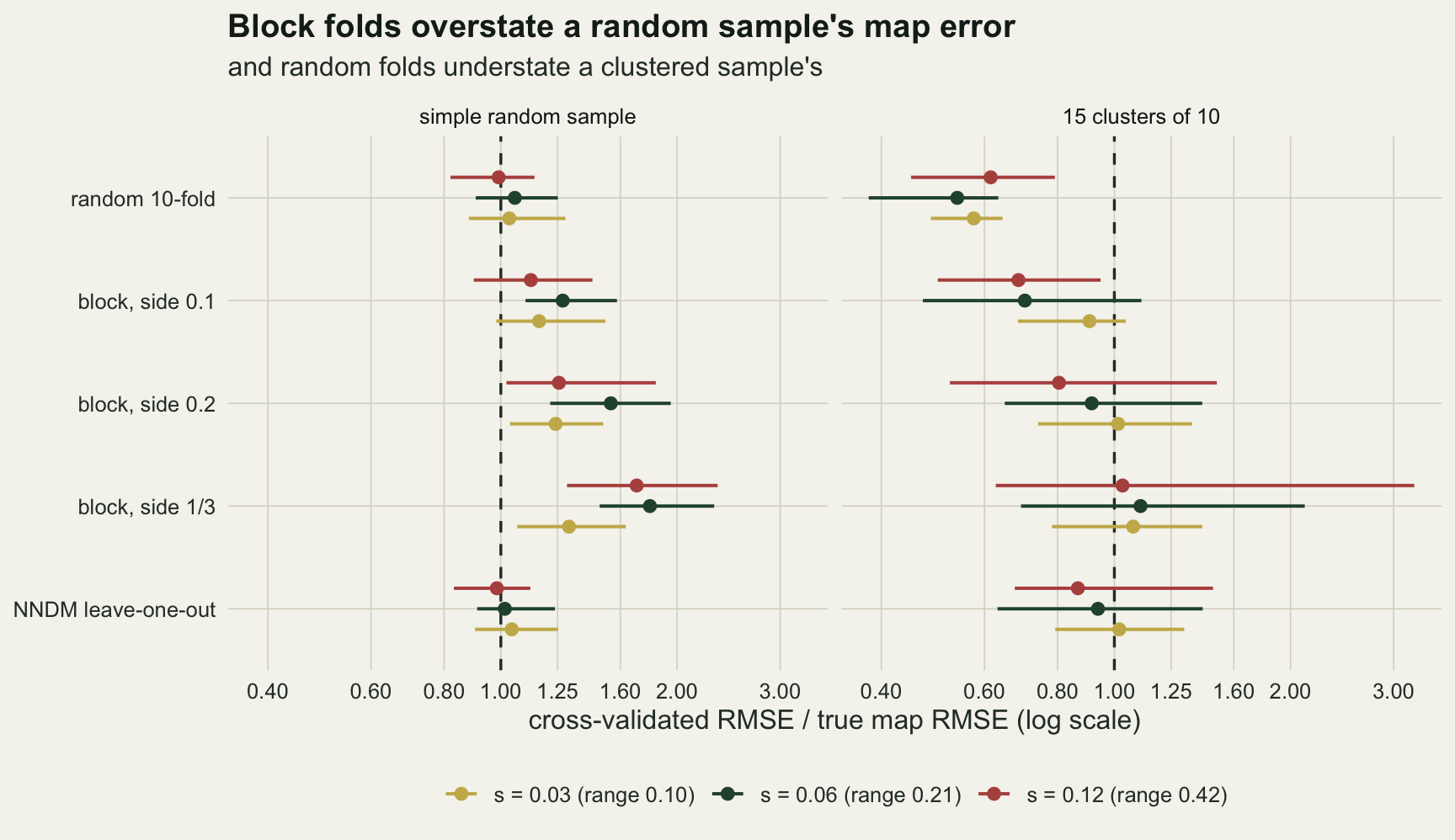
Block side against the range
The rule for block size that most readers carry is the one in the spatial cross-validation post: set the block side near the autocorrelation range. On a random sample with a map as the target, that advice fixes the size of the overshoot rather than removing it, and the size depends on more than the ratio of side to range.
sweep_tab <- do.call(rbind, lapply(s_vals, function(s_ker) {
  cl <- paste(s_ker, "random")
  ks <- if (s_ker == s_head) k_sweep else c(10, 5, 3)
  do.call(rbind, lapply(ks, function(k) {
    v <- ratio_of(cl, paste0("blk", k))
    data.frame(s_ker = s_ker, side = 1 / k, rel = (1 / k) / range_05[as.character(s_ker)],
               med = median(v), lo = min(v), hi = max(v))
  }))
}))
at_range <- ratio_of("0.03 random", "blk10")
rel_short <- (1 / 10) / range_05["0.03"]
half_06 <- sweep_tab[sweep_tab$s_ker == 0.06 & sweep_tab$side == 1 / 10, ]
half_12 <- sweep_tab[sweep_tab$s_ker == 0.12 & sweep_tab$side == 1 / 5, ]
true_gain_frac <- sapply(s_vals, function(s_ker) {
  m <- cells[[paste(s_ker, "random")]]
  median(1 - m[, "rk_truth"] / m[, "lm_truth"])
})
lm_blk5 <- sapply(s_vals, function(s_ker) median(ratio_of(paste(s_ker, "random"), "blk5", "lm")))
At s = 0.06 the overshoot climbs steadily with the block side, from 1.24 at side 1/12 to 1.80 at side 1/3 (medians). At a side of about half the range the two longer scales agree: side 0.1 at s = 0.06 reads 1.28 and side 0.2 at s = 0.12 reads 1.26. At a side equal to the range they do not. Side 0.1 at s = 0.03, which is 0.96 ranges, reads only 1.16 [0.98, 1.51], against 1.54 for the matching side at s = 0.06.
The difference is how much the spatial term is worth in the first place. On the true map, kriging the residuals removes a median 21 per cent of the least squares error at s = 0.03, 45 per cent at s = 0.06 and 53 per cent at s = 0.12. Almost all of the overshoot sits in the kriging step: least squares alone, scored the same way with block side 0.2, reads 1.03, 1.06 and 1.09 of its own true map error at the three scales. So where the residual field is fine-grained compared with the spacing of 150 plots, kriging adds little and blocking has little to take away. Any overshoot figure is a property of the side, the range and (untested here) the sampling density together, and the next section reads it in the unit that matters to the analyst.
sweep_tab$s_f <- factor(sprintf("s = %.2f", sweep_tab$s_ker))
ggplot(sweep_tab, aes(rel, med, colour = s_f)) +
  geom_hline(yintercept = 1, linetype = "dashed", colour = te_body, linewidth = 0.6) +
  geom_vline(xintercept = 1, linetype = "dotted", colour = te_body, linewidth = 0.6) +
  geom_errorbar(aes(ymin = lo, ymax = hi), width = 0, linewidth = 0.6, alpha = 0.7) +
  geom_line(linewidth = 0.8) +
  geom_point(size = 2.3) +
  scale_x_log10(breaks = c(0.25, 0.5, 1, 2, 3)) +
  scale_colour_manual(values = c(te_gold, te_forest, te_rust), name = NULL) +
  labs(x = "block side / residual range (log scale)",
       y = "block CV RMSE / true map RMSE",
       title = "The overshoot grows with the block side",
       subtitle = "random design; dotted line: side equal to the range") +
  theme_datasheet() +
  theme(legend.position = "bottom")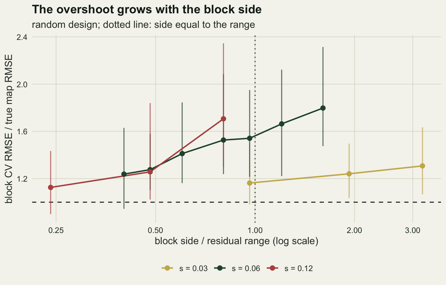
The spatial term a block scheme erases
A validation number is rarely reported alone. It is usually one of two numbers, the error with the spatial term and the error without it, and the difference is the evidence that the kriging step earns its place. The quantity that matters to the analyst is therefore the reported gain, the least squares error minus the regression-kriging error under a scheme, divided by the true gain on the map.
gain_tab <- do.call(rbind, lapply(names(cells), function(cl) {
  parts <- strsplit(cl, " ")[[1]]
  do.call(rbind, lapply(c("rand10", "blk5", "blk3", "nndm"), function(sc) {
    v <- gain_of(cl, sc)
    data.frame(s_ker = as.numeric(parts[1]), design = parts[2], scheme = sc,
               med = median(v), q1 = unname(quantile(v, 0.25)),
               q3 = unname(quantile(v, 0.75)))
  }))
}))
n_neg_b3 <- n_neg("0.06 clustered", "blk3")
nndm_gain_med <- sapply(paste(s_vals, "clustered"), function(cl) median(gain_of(cl, "nndm")))
On the random design, block side 0.2 reports 0.21 [-0.01, 0.67] of the true gain at s = 0.03 and 0.41 [0.18, 1.01] at s = 0.06; at s = 0.03 it reports a negative gain in 1 of 20 draws, so on that draw the reviewer’s scheme would have told her to drop a spatial term that was doing real work. Side 1/3 does worse, 0.14 and 0.27 in median. Random ten-fold reports medians of 0.85, 0.97 and 0.98 of the true gain at the three scales, and NNDM 0.85, 1.00 and 0.98.
On the clustered design random ten-fold inflates the gain, to a median 4.34 times the true value at s = 0.03, 2.30 at s = 0.06 and 1.22 at s = 0.12. The plots inside a cluster predict each other through the kriging term, so the term looks far more valuable than it is for the cells between clusters. NNDM reads 1.13 [0.44, 2.70], 1.04 [-0.04, 2.22] and 0.84 [0.44, 5.55]: medians between 0.84 and 1.13, wide in any single draw.
None of this is a ranking reversal in the usual sense. Every scheme prefers the kriging model in nearly every draw; the one place a scheme often picks the wrong model is block side 1/3 on the clustered sample at s = 0.06, which reports a negative gain in 8 of 40 draws. The common failure is quieter: a correct model choice carried by a gain that is often misstated by a factor of two or more, in a direction set by the sampling design.
gain_tab$scheme_f <- factor(scheme_lab[gain_tab$scheme], levels = rev(scheme_lab))
gain_tab$s_f <- factor(sprintf("s = %.2f", gain_tab$s_ker))
gain_tab$design_f <- factor(ifelse(gain_tab$design == "random", "simple random sample",
                                   "15 clusters of 10"),
                            levels = c("simple random sample", "15 clusters of 10"))
ggplot(gain_tab, aes(med, scheme_f, colour = s_f)) +
  geom_vline(xintercept = 1, linetype = "dashed", colour = te_body, linewidth = 0.6) +
  geom_vline(xintercept = 0, colour = te_line, linewidth = 0.8) +
  geom_errorbar(aes(xmin = q1, xmax = q3), orientation = "y", width = 0,
                linewidth = 0.7, position = position_dodge(width = 0.6)) +
  geom_point(size = 2.2, position = position_dodge(width = 0.6)) +
  facet_wrap(~ design_f) +
  scale_colour_manual(values = c(te_gold, te_forest, te_rust), name = NULL) +
  labs(x = "reported gain / true gain", y = NULL,
       title = "The kriging gain, misstated in both directions",
       subtitle = "dashed line: the gain the map really has") +
  theme_datasheet() +
  theme(legend.position = "bottom")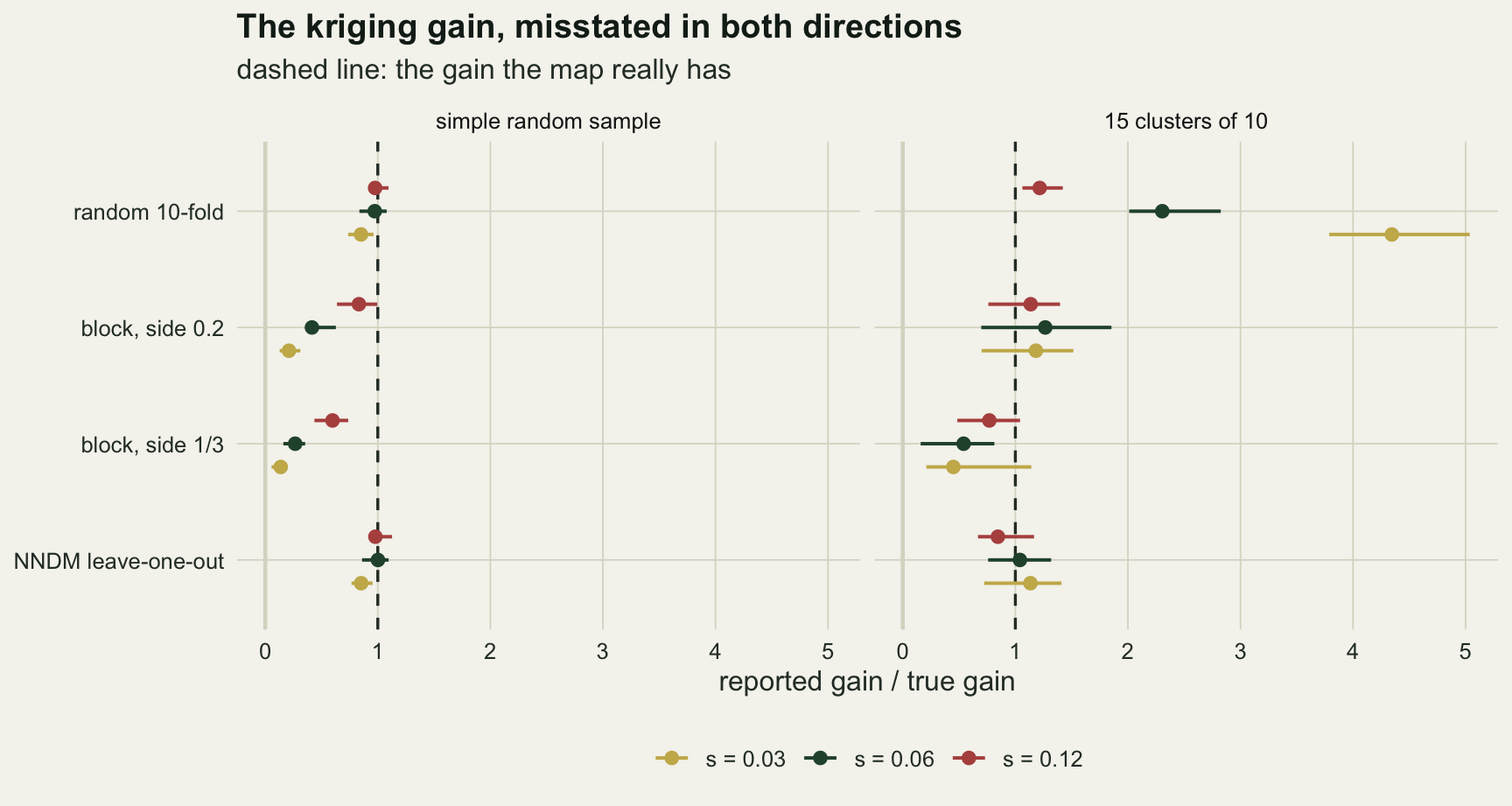
The check to run before any fold is drawn
Everything above follows from one comparison, and that comparison needs only the coordinates. A scheme scores each held-out plot at the distance to training data the scheme leaves it; the map’s error is set by the distances from the prediction cells to the sample. Plotting the two empirical distribution functions on one panel shows which scheme matches the map before any model is fitted.
set.seed(606)
ecdf_list <- lapply(c("random", "clustered"), function(des) {
  idx  <- draw_sample(des)
  xy   <- xy_all[idx, ]
  pc   <- setdiff(seq_len(n_cell), idx)
  dmat <- as.matrix(dist(xy))
  gpred <- apply(cross_dist(xy_all[pc, ], xy), 1, min)
  fl <- list(rand10 = random_folds(n_samp), blk5 = block_folds(xy, 5),
             nndm = nndm_folds(dmat, gpred))
  lab <- if (des == "random") "simple random sample" else "15 clusters of 10"
  rows <- rbind(data.frame(design = lab, curve = "prediction cells to sample", d = gpred),
                do.call(rbind, lapply(names(fl), function(nm)
                  data.frame(design = lab, curve = scheme_lab[[nm]], d = test_nn(fl[[nm]], dmat)))))
  list(rows = rows, w = sapply(fl, function(f) w_stat(test_nn(f, dmat), gpred)),
       med_pred = median(gpred), med_r10 = median(test_nn(fl$rand10, dmat)),
       med_b5 = median(test_nn(fl$blk5, dmat)))
})
ecdf_rows <- do.call(rbind, lapply(ecdf_list, `[[`, "rows"))
w_ran <- ecdf_list[[1]]$w
w_clu <- ecdf_list[[2]]$w
On the random draw shown, the median distance from a cell to its nearest plot is 0.035; random ten-fold leaves each held-out plot a median 0.044 from its nearest training plot, and block side 0.2 leaves 0.091. On the clustered draw the cells sit a median 0.078 from the nearest plot, while random ten-fold leaves a held-out plot only 0.022 from a training plot in its own cluster. The areas between the curves say the same in one number each: 0.0030 for random ten-fold and 0.0510 for block side 0.2 on the random draw, 0.0674 and 0.0217 on the clustered one. NNDM, which builds the match, gets 0.0010 and 0.0016.
curve_lev <- c("prediction cells to sample", scheme_lab[c("rand10", "blk5", "nndm")])
ecdf_rows$curve <- factor(ecdf_rows$curve, levels = curve_lev)
ecdf_rows$design <- factor(ecdf_rows$design, levels = c("simple random sample", "15 clusters of 10"))
ggplot(ecdf_rows, aes(d, colour = curve, linetype = curve)) +
  stat_ecdf(linewidth = 0.9, pad = FALSE) +
  facet_wrap(~ design, scales = "free_x") +
  scale_colour_manual(values = c(te_ink, te_gold, te_forest, te_rust), name = NULL) +
  scale_linetype_manual(values = c("solid", "solid", "solid", "22"), name = NULL) +
  labs(x = "distance to the nearest sample or training plot (map side = 1)",
       y = "cumulative proportion",
       title = "Match the black curve before choosing a scheme",
       subtitle = "one draw per design; a scheme whose curve lies on the black one reads the map error") +
  theme_datasheet() +
  theme(legend.position = "bottom") +
  guides(colour = guide_legend(nrow = 2), linetype = guide_legend(nrow = 2))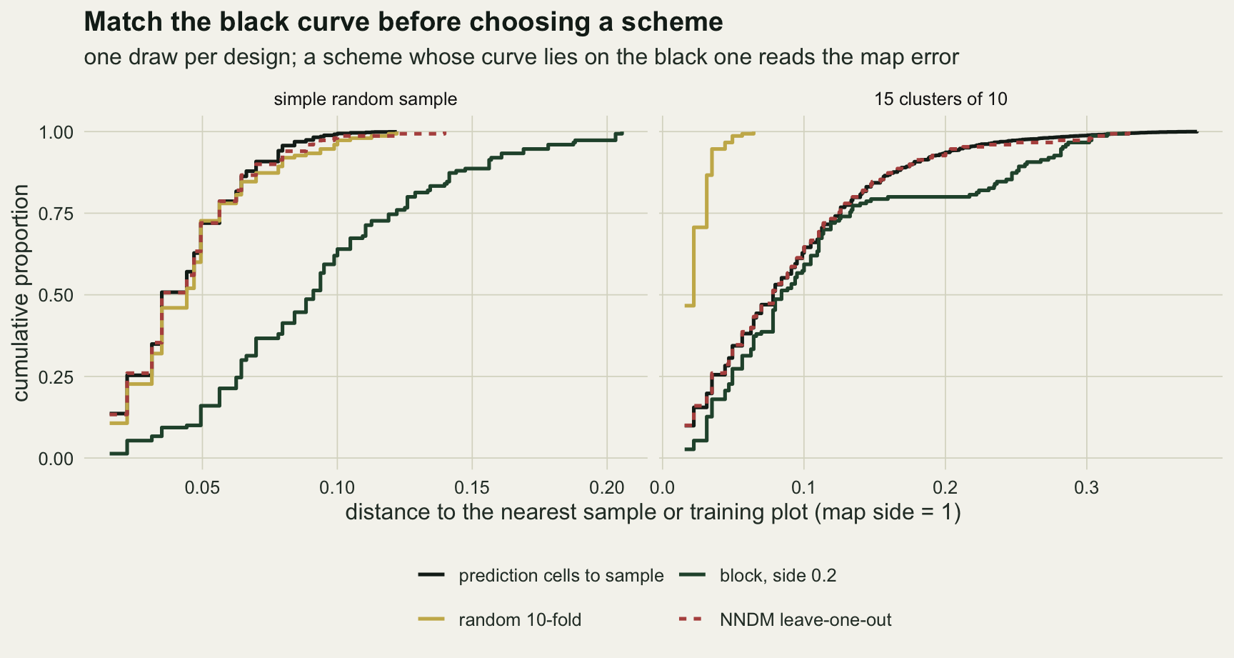
The figure is one draw. Whether the check picks the right scheme in general can be measured on all the draws above, because every draw stored its distance statistic for every scheme. The rule tested is the one a reader can apply: among the ready-made schemes (random ten-fold and the three block sides), take the one with the smallest area between the curves.
fixed_sc <- c("rand10", "blk10", "blk5", "blk3")
pick_by_w <- function(cl) {
  m <- cells[[cl]]
  w_m <- m[, paste0("W_", fixed_sc), drop = FALSE]
  r_m <- m[, paste0("rk_", fixed_sc), drop = FALSE] / m[, "rk_truth"]
  chosen <- apply(w_m, 1, which.min)
  best   <- apply(abs(log(r_m)), 1, which.min)
  list(ratio = r_m[cbind(seq_len(nrow(r_m)), chosen)],
       agree = mean(chosen == best),
       top = names(which.max(table(fixed_sc[chosen]))),
       top_share = max(table(chosen)) / length(chosen),
       chosen = fixed_sc[chosen], best = fixed_sc[best])
}
pick <- lapply(setNames(names(cells), names(cells)), pick_by_w)
pick_ran <- unlist(lapply(pick[grep("random", names(pick))], `[[`, "ratio"))
pick_clu <- lapply(pick[grep("clustered", names(pick))], `[[`, "ratio")
top_clu <- sapply(pick[grep("clustered", names(pick))], `[[`, "top")
stopifnot(all(top_clu == "blk5"))
top_clu_share <- sapply(pick[grep("clustered", names(pick))], `[[`, "top_share")
chosen_clu <- unlist(lapply(pick[grep("clustered", names(pick))], `[[`, "chosen"))
n_r10_clu <- sum(chosen_clu == "rand10")
n_clu_draws <- length(chosen_clu)
agree_clu <- sapply(pick[grep("clustered", names(pick))], `[[`, "agree")
n_ran_draws <- length(pick_ran)
# the widest pick on the clustered design, and the draws where the pick is not the best scheme
exc_i     <- which.max(pick[["0.06 clustered"]]$ratio)
exc_sc    <- pick[["0.06 clustered"]]$chosen[exc_i]
exc_ratio <- pick[["0.06 clustered"]]$ratio[exc_i]
exc_nndm  <- ratio_of("0.06 clustered", "nndm")[exc_i]
stopifnot(exc_ratio > max(pick_clu[[1]], pick_clu[[3]]), exc_sc == "blk3")
ch_clu <- unlist(lapply(pick[grep("clustered", names(pick))], `[[`, "chosen"))
be_clu <- unlist(lapply(pick[grep("clustered", names(pick))], `[[`, "best"))
n_dis    <- sum(ch_clu != be_clu)
n_dis_bb <- sum(ch_clu != be_clu & grepl("blk", ch_clu) & grepl("blk", be_clu))
stopifnot(n_dis_bb == n_dis)
n_r10_ran <- sum(unlist(lapply(pick[grep("random", names(pick))], `[[`, "chosen")) == "rand10")
On the random design the rule picks random ten-fold in 80 of 80 draws, and the number it picks reads 1.02 [0.82, 1.29] of the truth across them. On the clustered design it picks block side 0.2 most often, in 60 to 78 per cent of draws depending on the scale, and random ten-fold in 0 of 80 clustered draws. The number it picks reads 1.06 [0.75, 1.41], 0.90 [0.65, 2.11] and 0.92 [0.69, 1.50] at the three scales. The systematic understatement of random ten-fold is gone, and what remains is a scatter of the same order as NNDM’s, with one wider excursion at s = 0.06, a draw where the rule chose block side 1/3 and read 2.11 while NNDM read 1.41: with at most nine blocks dealt to five folds, one fold can hold out several clusters at once.
The check does not find the best scheme draw by draw. Among the four ready-made schemes it names the one closest to the truth in only 35 to 60 per cent of clustered draws, and in every one of the 46 draws where it misses, both the scheme it names and the best one are block sides. What it does is refuse the scheme that is wrong in a known direction, on either design, using nothing but the coordinates of the plots and of the cells to be mapped.
A fitted kernel instead of the known one
The kriging above was given the process covariance. In a real analysis the kernel is estimated, and a fair question is whether the ratios survive the estimation noise. At s = 0.06 every draw also fitted the kernel standard deviation, the sill and the nugget by maximum likelihood over a grid, from the least squares residuals of the whole sample, and then ran the headline schemes with the fitted kernel. The fit is made once, outside the folds, which is how most analyses do it and is itself a small leak.
s_hat_ran <- cells[["0.06 random"]][, "s_hat"]
s_hat_clu <- cells[["0.06 clustered"]][, "s_hat"]
The fitted kernel standard deviation has a median of 0.055 on the random design and 0.055 on the clustered one, against the true 0.06, with draws from 0.036 to 0.097. With it, the random design reads 1.04 [0.90, 1.25] for random ten-fold, 1.50 [1.22, 1.94] for block side 0.2 and 1.02 [0.87, 1.23] for NNDM; the clustered design reads 0.52 [0.38, 0.63], 0.90 [0.61, 1.39] and 0.94 [0.56, 1.42]. The median ratios move by a few hundredths at most. Part of the reason is that the truth is recomputed with the same fitted kernel, so a worse kernel moves both numbers together.
What to report
Say which error the number estimates. For a published map that is the error over the cells of the map, and it is the denominator every choice above was judged against. A number from a scheme that answers a different question (extrapolation to a new region, prediction of a new visit to a known site) belongs in the report only with that question attached.
If the plots are a probability sample, say so and use it. A simple random or stratified sample supports a design-based estimate of map accuracy, from an independent probability validation sample or, when the calibration plots are themselves the probability sample, from ordinary random cross-validation of them; no spatial blocking is needed, which is the recommendation of Wadoux and colleagues. Here, random ten-fold on a simple random sample landed close to the true map error and block cross-validation did not.
If the plots are not a probability sample, draw the two distance distributions before choosing a scheme and publish the figure. It costs a distance matrix, needs no model, and tells the reader why the scheme was chosen. Where no ready-made scheme matches, use NNDM leave-one-out, and report its spread honestly: with the fifteen clusters simulated here a single NNDM number was 0.94 [0.63, 1.42] of the truth across draws, so it is close to the truth in the median, with a wide error in any one survey.
Report the gain from the spatial term under the chosen scheme, not under a default. The size of that gain is what decides whether the kriging step appears in the methods section, and on a random sample a block scheme reported 0.41 of it in median at the medium range.
Honest limits
The kriging kernel is the process one in every arm except the fitted-kernel check, which was run only at s = 0.06 and fitted the kernel once, outside the folds. The covariance is Gaussian, the model is one linear trend plus simple kriging, and the covariates are smooth and cover the map; none of the numbers is a claim about random forests, generalised additive models or any other learner, only about the mechanism, which works through distances and is expected to carry over, though that is not tested.
The distance check looks only at the nearest neighbour, while kriging uses many neighbours. Whether a richer summary of the distances would name the best scheme more often draw by draw is not tested here.
Fifteen clusters give roughly fifteen pieces of information about the residual field, and the NNDM spread reported above is the price of that, not a coding fault. CAST also offers a k-fold version of the same distance matching; it was not run here, so whether it narrows the spread at fifteen clusters is untested. The NNDM function is a port of the loop in CAST::nndm() checked against the package source line by line, not a run of the package itself.
The prediction set is every unsampled cell of the map, known exactly. With presence-only data the prediction set is still the cells where the map will be read, but the model is fitted to presences and background points, and whether the distance comparison still picks the honest scheme once background sampling is part of the design is not tested here. Neither is extrapolation: a sample confined to half the map asks a question about new ground that no resampling of the sample can fully answer, and the distance comparison would show that as a black curve no scheme can reach.
The design-based estimate from an independent probability validation sample is described, not simulated. Wadoux and colleagues found standard cross-validation less biased than the spatial kind even on a strongly clustered biomass dataset with large differences in sampling density; the clustered design here is more extreme, every plot sitting in one of fifteen compact clusters, and on it the blocked schemes did better than random folds, so the two results describe different designs rather than contradicting each other. The ranges in brackets are the smallest and largest of 40 or 20 draws, so they widen with more draws, and the per-draw agreement percentages rest on the same small counts.
References
Wadoux AMJ-C, Heuvelink GBM, de Bruin S, Brus DJ 2021 Ecological Modelling 457:109692 (10.1016/j.ecolmodel.2021.109692)
Mila C, Mateu J, Pebesma E, Meyer H 2022 Methods in Ecology and Evolution 13(6):1304-1316 (10.1111/2041-210X.13851)
Ploton P, Mortier F, Rejou-Mechain M et al 2020 Nature Communications 11:4540 (10.1038/s41467-020-18321-y)