Tajima’s D and the frequency spectrum

Build Tajima’s D from the site frequency spectrum in R and measure what it detects: growth, structure and bottlenecks all move it, and so does selection.

The previous tutorial left two estimators of the same parameter which weight different parts of the gene tree: segregating sites use the whole tree, pairwise differences are dominated by its deep branches. If the tree has the shape the neutral constant-size model predicts, the two agree on average. If it does not, they disagree, and the direction of the disagreement says something about the shape.

Tajima’s D is that disagreement, divided by its standard deviation so that it can be compared across loci. This tutorial builds it, measures its distribution under neutrality, and then breaks the model in three ways to see what D does.

D from the spectrum

The statistic is (pi - theta_W) over the square root of its variance, and the variance expression is a page of algebra in the original paper that reduces to two constants multiplied by the number of segregating sites.

library(ggplot2)

te_pal <- list(forest = "#275139", green = "#2f8f63", sage = "#93a87f",
               clay = "#b5534e", gold = "#cda23f", line = "#dad9ca",
               ink = "#16241d")

theme_te <- function() {
  theme_minimal(base_size = 12) +
    theme(panel.grid.minor = element_blank(),
          panel.grid.major = element_line(colour = "#e7e6dc"),
          plot.background = element_rect(fill = "white", colour = NA),
          panel.background = element_rect(fill = "white", colour = NA),
          plot.title = element_text(face = "bold", colour = te_pal$ink),
          axis.title = element_text(colour = "#2c3a31"))
}

coal_branches <- function(n, size_fun = NULL, dt = 0.002, t_max = 20) {
  counts <- rep(1L, n)
  lens <- rep(0, n)
  out <- NULL
  if (is.null(size_fun)) {
    while (length(counts) > 1) {
      k <- length(counts)
      lens <- lens + rexp(1, rate = k * (k - 1) / 2)
      pick <- sample(k, 2)
      out <- rbind(out, cbind(counts[pick], lens[pick]))
      counts <- c(counts[-pick], sum(counts[pick]))
      lens <- c(lens[-pick], 0)
    }
  } else {
    t_now <- 0
    while (length(counts) > 1 && t_now < t_max) {
      k <- length(counts)
      if (runif(1) < k * (k - 1) / 2 / size_fun(t_now) * dt) {
        pick <- sample(k, 2)
        out <- rbind(out, cbind(counts[pick], lens[pick]))
        counts <- c(counts[-pick], sum(counts[pick]))
        lens <- c(lens[-pick], 0)
      }
      lens <- lens + dt
      t_now <- t_now + dt
    }
  }
  colnames(out) <- c("descendants", "length")
  out
}

sfs_from_tree <- function(br, n, theta) {
  muts <- rpois(nrow(br), theta / 2 * br[, "length"])
  tabulate(rep(br[, "descendants"], muts), nbins = n - 1)
}

stats_sfs <- function(sfs, n) {
  i <- seq_along(sfs)
  a1 <- sum(1 / seq_len(n - 1))
  a2 <- sum(1 / seq_len(n - 1)^2)
  s_tot <- sum(sfs)
  pi_hat <- sum(sfs * 2 * i * (n - i)) / (n * (n - 1))
  theta_w <- s_tot / a1
  b1 <- (n + 1) / (3 * (n - 1))
  b2 <- 2 * (n^2 + n + 3) / (9 * n * (n - 1))
  e1 <- (b1 - 1 / a1) / a1
  e2 <- (b2 - (n + 2) / (a1 * n) + a2 / a1^2) / (a1^2 + a2)
  vd <- e1 * s_tot + e2 * s_tot * (s_tot - 1)
  c(S = s_tot, pi = pi_hat, theta_w = theta_w,
    D = if (s_tot > 1 && vd > 0) (pi_hat - theta_w) / sqrt(vd) else NA)
}

The size_fun argument is what makes the histories below possible: pass a function giving population size relative to the present at time t in the past, and the coalescence rate is divided by it. A small population in the past coalesces faster.

Three broken models

Constant size is the null. Exponential growth means the population was smaller in the past, so lineages coalesce quickly once you look back far enough, producing star-like trees with many singletons. A bottleneck squeezes coalescence into a short window. Simulate 1500 loci of each with 20 sequences and theta = 5.

set.seed(484)
n <- 20
theta <- 5

grow <- function(alpha) function(t) exp(-alpha * t)
bott <- function(depth, t0, t1) function(t) if (t > t0 && t < t1) depth else 1

scen <- list(constant = NULL, growth = grow(5),
             bottleneck = bott(0.1, 0.05, 0.2))

d_all <- list()
d_tab <- NULL
for (nm in names(scen)) {
  vals <- t(replicate(1500, stats_sfs(
    sfs_from_tree(coal_branches(n, size_fun = scen[[nm]]), n, theta), n)))
  d_all[[nm]] <- vals[, "D"]
  d_tab <- rbind(d_tab, data.frame(
    history = nm, mean_S = round(mean(vals[, "S"]), 2),
    mean_pi = round(mean(vals[, "pi"]), 3),
    mean_D = round(mean(vals[, "D"], na.rm = TRUE), 3),
    frac_below_minus2 = round(mean(vals[, "D"] < -2, na.rm = TRUE), 4),
    frac_above_2 = round(mean(vals[, "D"] > 2, na.rm = TRUE), 4)))
}
print(d_tab, row.names = FALSE)

    history mean_S mean_pi mean_D frac_below_minus2 frac_above_2
   constant  17.35   4.834 -0.115            0.0120       0.0153
     growth   6.72   1.475 -0.702            0.0114       0.0013
 bottleneck   6.34   1.727 -0.383            0.0287       0.0398

Under constant size the mean D is -0.115, close to zero but not exactly zero: the statistic is standardised, not centred, and a small negative mean at this sample size is expected rather than a bug. The tails are 1.2 percent below -2 and 1.53 percent above +2, so the conventional cutoffs behave roughly like a five percent two-sided test.

Exponential growth pushes the mean to -0.702 and empties the upper tail (0.13 percent above +2). It also cuts diversity hard, mean pi from 4.834 to 1.475, because a population that was small in the past has a shallow tree. The bottleneck does something more interesting: the mean moves only to -0.383, but both tails get fatter, 2.87 percent below -2 and 3.98 percent above +2 against 1.2 and 1.53 under neutrality. A bottleneck is a lottery over which lineages survive it, and depending on the draw a locus can come out looking either star-like or deeply split.

The case that produces positive D

For a consistently positive D the usual culprit is not a bottleneck but population structure. Sample from two demes with limited migration and the deep split between them adds intermediate-frequency variants, which is what pi weights most.

coal_struct <- function(n_per_deme, m_scaled, dt = 0.002, t_max = 40) {
  deme <- rep(1:2, each = n_per_deme)
  counts <- rep(1L, 2 * n_per_deme)
  lens <- rep(0, length(counts))
  out <- NULL
  t_now <- 0
  while (length(counts) > 1 && t_now < t_max) {
    for (d in 1:2) {
      idx <- which(deme == d)
      k <- length(idx)
      if (k >= 2 && runif(1) < k * (k - 1) / 2 * 2 * dt) {
        pick <- sample(idx, 2)
        out <- rbind(out, cbind(counts[pick], lens[pick]))
        counts <- c(counts[-pick], sum(counts[pick]))
        lens <- c(lens[-pick], 0)
        deme <- c(deme[-pick], d)
      }
    }
    mig <- runif(length(counts)) < m_scaled / 2 * dt
    if (any(mig)) deme[mig] <- 3 - deme[mig]
    lens <- lens + dt
    t_now <- t_now + dt
  }
  colnames(out) <- c("descendants", "length")
  out
}

set.seed(485)
struct_tab <- NULL
for (m_scaled in c(0.2, 1, 5)) {
  vals <- t(replicate(400, stats_sfs(
    sfs_from_tree(coal_struct(10, m_scaled), n, theta), n)))
  d_all[[paste("structure, M =", m_scaled)]] <- vals[, "D"]
  struct_tab <- rbind(struct_tab, data.frame(
    M = m_scaled, mean_S = round(mean(vals[, "S"]), 2),
    mean_pi = round(mean(vals[, "pi"]), 3),
    mean_D = round(mean(vals[, "D"], na.rm = TRUE), 3),
    frac_above_2 = round(mean(vals[, "D"] > 2, na.rm = TRUE), 4)))
}
print(struct_tab, row.names = FALSE)

   M mean_S mean_pi mean_D frac_above_2
 0.2  42.90  17.112  1.359        0.345
 1.0  24.05   7.755  0.450        0.075
 5.0  18.67   5.320 -0.039        0.015

With M = 4Nm of 0.2, meaning one migrant every few generations across the whole metapopulation, mean D is +1.359 and 34.5 percent of loci exceed +2. Diversity is inflated too, pi of 17.112 against 4.834 for a single panmictic population of the same local size, because the sample spans two histories. Raise migration to M = 1 and the effect halves (mean D +0.45); at M = 5 it is gone (-0.039), which is the same threshold behaviour the Fst tutorial found from the forward direction.

show <- c("constant", "growth", "bottleneck", "structure, M = 0.2",
          "structure, M = 1")
dist_df <- do.call(rbind, lapply(show, function(nm)
  data.frame(D = d_all[[nm]], history = nm)))
dist_df$history <- factor(dist_df$history, levels = show)

ggplot(subset(dist_df, !is.na(D)), aes(D, colour = history)) +
  geom_vline(xintercept = c(-2, 2), linetype = "dashed",
             colour = te_pal$line) +
  geom_density(linewidth = 0.9) +
  scale_colour_manual(values = c(constant = te_pal$ink, growth = te_pal$clay,
                                 bottleneck = te_pal$gold,
                                 `structure, M = 0.2` = te_pal$forest,
                                 `structure, M = 1` = te_pal$sage),
                      name = NULL) +
  labs(title = "Demography moves Tajima's D in both directions",
       subtitle = "1500 loci per history for the first three, 400 for the structured ones",
       x = "Tajima's D", y = "density") +
  theme_te()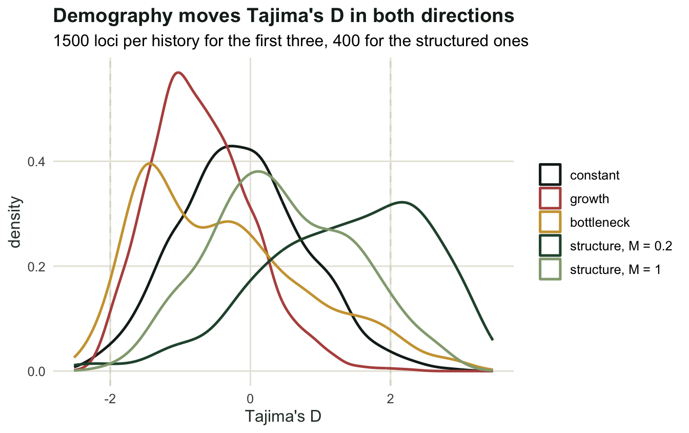

Figure 1: Distributions of Tajima’s D across simulated loci under five histories, with the conventional cutoffs at plus and minus two.

What this means for reading D

The table above is the reason a single significant D is not evidence of selection. A negative D is produced by a selective sweep, which drags a star-like genealogy behind it, and it is equally produced by population growth, which does the same thing genome-wide. A positive D is produced by balancing selection, and it is equally produced by unrecognised population structure, by admixture, and by a bottleneck that happened to split the sample.

Three practical consequences.

First, D is a relative statistic in practice. What identifies a candidate locus is not its D value but its position in the genome-wide distribution of D, because demography shifts that whole distribution while selection acts on individual loci. A locus at D = -2.5 in a genome whose median is -0.7 is unremarkable; the same value in a genome centred on zero is worth a look.

Second, the sign carries more information than the magnitude when the direction is diagnostic. A study that finds a mean D of -0.7 across hundreds of loci has evidence about the population’s history, not about hundreds of sweeps.

Third, the same demographic simulation that shifts D also shifts diversity, and the two together constrain the history better than either alone. Growth here cut pi to a third while making D negative; structure inflated pi more than threefold while making D positive. Reporting both makes those two histories distinguishable, and reporting D alone does not.

Where to go next

The last tutorial in the cluster turns this into a set of checks: how much a single locus can say, what recombination does to the variance, whether growth and a sweep can be separated at all from a frequency spectrum, and where the coalescent model itself stops being a reasonable description.

References

Tajima F 1989 Genetics 123(3):585-595 (10.1093/genetics/123.3.585)

Simonsen KL, Churchill GA, Aquadro CF 1995 Genetics 141(2):413-429 (10.1093/genetics/141.2.413)

Nielsen R 2005 Annual Review of Genetics 39:197-218 (10.1146/annurev.genet.39.073003.112420)

Stajich JE, Hahn MW 2005 Molecular Biology and Evolution 22(1):63-73 (10.1093/molbev/msh252)

Related tutorials

• The coalescent and gene trees
• Nucleotide diversity and Watterson theta
• Checking a coalescent analysis
• Checking a population genetics analysis