The coalescent and gene trees

Simulate the coalescent in R, check the tree height and total branch length against theory, and see why a single gene tree says almost nothing about history.

Everything in this cluster so far has run forwards: start with a population, let drift and mutation act, see what the sample looks like. The coalescent runs the same process backwards. Take the sample, trace ancestral lineages until they meet, and you get a gene tree whose shape carries the demographic history that produced it.

The backward view is not just an alternative; it is what makes computation cheap. A Wright-Fisher simulation has to track a whole population to say something about ten sampled gene copies. The coalescent tracks the ten lineages and nothing else, and one line of rexp() does it.

Waiting for a coalescence

With k ancestral lineages in a population of 2N gene copies, any particular pair shares a parent in the previous generation with probability 1/(2N), and there are k(k-1)/2 pairs. Measure time in units of 2N generations and the waiting time until the next coalescence is exponential with rate k(k-1)/2. That is the whole model.

library(ggplot2)

te_pal <- list(forest = "#275139", green = "#2f8f63", sage = "#93a87f",
               clay = "#b5534e", gold = "#cda23f", line = "#dad9ca",
               ink = "#16241d")

theme_te <- function() {
  theme_minimal(base_size = 12) +
    theme(panel.grid.minor = element_blank(),
          panel.grid.major = element_line(colour = "#e7e6dc"),
          plot.background = element_rect(fill = "white", colour = NA),
          panel.background = element_rect(fill = "white", colour = NA),
          plot.title = element_text(face = "bold", colour = te_pal$ink),
          axis.title = element_text(colour = "#2c3a31"))
}

coal_times <- function(n) {
  k <- n:2
  rexp(length(k), rate = k * (k - 1) / 2)
}

tmrca <- function(n) sum(coal_times(n))

total_len <- function(n) {
  k <- n:2
  sum(rexp(length(k), rate = k * (k - 1) / 2) * k)
}

set.seed(477)
reps <- 20000
n_grid <- c(2, 5, 10, 20, 50)
tab <- t(sapply(n_grid, function(n) {
  tt <- replicate(reps, tmrca(n))
  tl <- replicate(reps, total_len(n))
  c(n = n, tmrca_sim = mean(tt), tmrca_theory = 2 * (1 - 1 / n),
    tmrca_sd = sd(tt), total_sim = mean(tl),
    total_theory = 2 * sum(1 / seq_len(n - 1)))
}))
print(round(tab, 3))

      n tmrca_sim tmrca_theory tmrca_sd total_sim total_theory
[1,]  2     1.006         1.00    0.990     2.035        2.000
[2,]  5     1.606         1.60    1.076     4.176        4.167
[3,] 10     1.806         1.80    1.092     5.624        5.658
[4,] 20     1.891         1.90    1.077     7.084        7.095
[5,] 50     1.961         1.96    1.073     8.948        8.958

Two expectations fall out of the exponential waiting times, and the simulation reproduces both. The time to the most recent common ancestor is 2(1 - 1/n) in units of 2N generations, so 1.006 against 1.000 for a pair and 1.961 against 1.960 for fifty lineages. The total branch length is 2 * sum(1/k) for k from 1 to n-1, giving 8.948 against 8.958 at n = 50.

Look at how differently those two quantities grow. Going from two samples to fifty roughly doubles the tree height, from 1.0 to 1.96, and it can never exceed 2 no matter how many individuals are sequenced. The total branch length grows without bound, but only logarithmically: 2.0, 4.167, 5.658, 7.095, 8.958. Mutations accumulate in proportion to total branch length, so this is the coalescent statement of the sampling result from the previous tutorial: the tenth individual adds a lot, the fiftieth adds very little, and neither adds much depth.

One tree is one draw

The standard deviation column is the part that gets forgotten. At n = 10 the mean TMRCA is 1.806 and the standard deviation is 1.092.

set.seed(478)
n_show <- 10
parts <- t(replicate(5000, {
  ts <- coal_times(n_show)
  c(t2_share = ts[length(ts)] / sum(ts), tmrca = sum(ts))
}))

cat("mean share of the tree height spent with two lineages:",
    round(mean(parts[, "t2_share"]), 4),
    " ratio of expectations 1/(2(1 - 1/n)):",
    round(1 / (2 * (1 - 1 / n_show)), 4), "\n")

mean share of the tree height spent with two lineages: 0.4683  ratio of expectations 1/(2(1 - 1/n)): 0.5556 

cat("TMRCA coefficient of variation at n = 10:",
    round(sd(parts[, "tmrca"]) / mean(parts[, "tmrca"]), 4), "\n")

TMRCA coefficient of variation at n = 10: 0.604 

A coefficient of variation of 0.604 means the tree height for one locus is essentially a single draw from a very broad distribution. Two loci with the same demographic history can easily differ threefold in depth, and no amount of extra sampling within a locus fixes that, because all the sampled copies share the same tree. This is the deepest structural reason why population genetic inference needs many independent loci rather than deep sampling of a few.

The other number explains the shape of every gene tree you will ever draw. The interval during which only two lineages remain has expectation 1, out of a total expectation of 1.806, so 0.5556 of the tree height sits in that last interval. Averaging the per-tree share rather than the expectations gives 0.4683, slightly lower because the ratio is not linear. Either way, roughly half the depth of a gene tree is one long stretch with two lineages, and the coalescences that separate the ten samples are crowded into the recent end.

set.seed(480)
`%||%` <- function(a, b) if (is.null(a)) b else a

draw_tree <- function(n) {
  x <- seq_len(n)
  active <- as.list(seq_len(n))
  height <- 0
  segs <- data.frame()
  pos <- x
  while (length(active) > 1) {
    k <- length(active)
    height <- height + rexp(1, rate = k * (k - 1) / 2)
    pick <- sample(k, 2)
    for (i in pick) {
      segs <- rbind(segs, data.frame(x = pos[i], xend = pos[i],
                                     y = attr(active[[i]], "h") %||% 0,
                                     yend = height))
    }
    segs <- rbind(segs, data.frame(x = pos[pick[1]], xend = pos[pick[2]],
                                   y = height, yend = height))
    new_pos <- mean(pos[pick])
    keep <- setdiff(seq_len(k), pick)
    merged <- structure(list(unlist(active[pick])), h = height)
    active <- c(active[keep], merged)
    pos <- c(pos[keep], new_pos)
    attr(active[[length(active)]], "h") <- height
  }
  segs
}
segs <- draw_tree(10)
cat("this tree: height", round(max(segs$yend), 3), "\n")

this tree: height 2.765 

ggplot(segs) +
  geom_segment(aes(x = x, xend = xend, y = y, yend = yend),
               colour = te_pal$forest, linewidth = 0.7) +
  labs(title = "A gene tree for ten sampled copies",
       subtitle = "coalescent units of 2N generations; time runs upward into the past",
       x = "sampled lineages", y = "time before the present") +
  theme_te() +
  theme(axis.text.x = element_blank(), panel.grid.major.x = element_blank())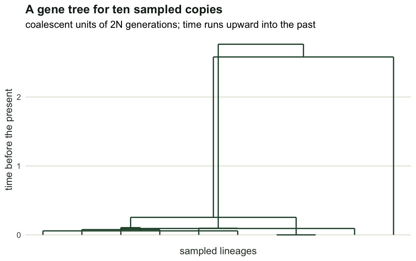

Figure 1: One realised coalescent tree for ten sampled lineages, drawn on the coalescent timescale. The final interval with two lineages takes up much of the height.

theory_df <- data.frame(n = 2:60)
theory_df$tmrca <- 2 * (1 - 1 / theory_df$n)
theory_df$total <- sapply(theory_df$n, function(n) 2 * sum(1 / seq_len(n - 1)))
long_theory <- rbind(
  data.frame(n = theory_df$n, value = theory_df$tmrca, what = "tree height"),
  data.frame(n = theory_df$n, value = theory_df$total,
             what = "total branch length"))
sim_df <- as.data.frame(tab)
long_sim <- rbind(
  data.frame(n = sim_df$n, value = sim_df$tmrca_sim, what = "tree height"),
  data.frame(n = sim_df$n, value = sim_df$total_sim,
             what = "total branch length"))

ggplot(long_theory, aes(n, value, colour = what)) +
  geom_line(linewidth = 0.9) +
  geom_point(data = long_sim, size = 2.4) +
  scale_x_log10(breaks = c(2, 5, 10, 20, 50)) +
  scale_colour_manual(values = c(`tree height` = te_pal$clay,
                                 `total branch length` = te_pal$forest),
                      name = NULL) +
  labs(title = "Depth saturates, branch length does not",
       subtitle = "lines: coalescent expectations, points: 20000 simulated trees per sample size",
       x = "sampled lineages (log scale)",
       y = "coalescent units of 2N generations") +
  theme_te()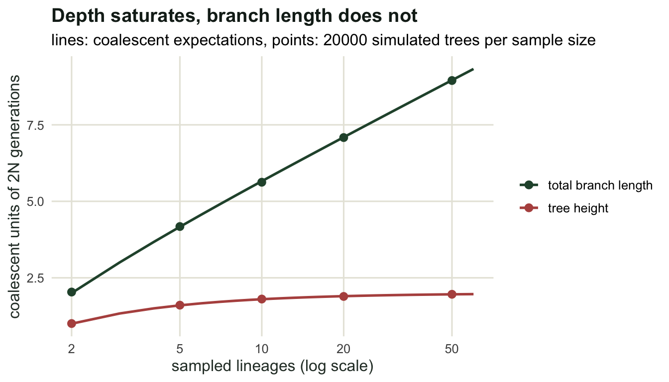

Figure 2: Tree height and total branch length against sample size, simulated against the coalescent expectations.

Does it match a real population?

The coalescent is an approximation to the Wright-Fisher model, valid when the sample is small relative to the population. It is worth checking that against the forward simulation the earlier tutorials used, rather than taking it on faith. Two gene copies in a population of N diploids should coalesce after a geometric number of generations with mean 2N.

set.seed(479)
wf_pair <- function(n_dip, max_gen = 20000) {
  for (g in seq_len(max_gen)) {
    pa <- sample(2 * n_dip, 1)
    pb <- sample(2 * n_dip, 1)
    if (pa == pb) return(g)
  }
  NA
}

n_dip <- 50
pair_times <- replicate(3000, wf_pair(n_dip))
cat("Wright-Fisher with N =", n_dip,
    ": mean pairwise coalescence time", round(mean(pair_times), 1),
    " expected 2N", 2 * n_dip, "\n")

Wright-Fisher with N = 50 : mean pairwise coalescence time 98.2  expected 2N 100 

cat("standard deviation", round(sd(pair_times), 1),
    " expected (geometric)", round(2 * n_dip, 1),
    " in coalescent units", round(mean(pair_times) / (2 * n_dip), 3), "\n")

standard deviation 96.6  expected (geometric) 100  in coalescent units 0.982 

Mean 98.2 generations against an expected 100, with a standard deviation of 96.6 against an expected 100: the geometric distribution has a standard deviation almost equal to its mean, which is where the exponential approximation comes from and why coalescence times are so variable. Dividing by 2N puts the forward simulation on the coalescent timescale at 0.982, and the two models agree.

That correspondence is what makes Ne usable in the coalescent. The backward process does not know about sex ratios or reproductive variance; it only knows a rate. Everything the previous tutorials did to Ne shows up here as a change of timescale, which is why coalescent methods estimate an effective size rather than a census.

Where to go next

A tree by itself is not data. What gets observed is mutations, and mutations fall on branches in proportion to their length, which turns the tree into a pattern of variable sites. The next tutorial adds mutation to these trees and derives the two classical diversity estimators, one counting differences between sequences and one counting segregating sites, then measures which is more precise and why.

References

Kingman JFC 1982 Stochastic Processes and their Applications 13(3):235-248 (10.1016/0304-4149(82)90011-4)

Hudson RR 1990 Oxford Surveys in Evolutionary Biology 7:1-44 (no DOI)

Rosenberg NA, Nordborg M 2002 Nature Reviews Genetics 3(5):380-390 (10.1038/nrg795)

Wakeley J 2009 Coalescent Theory: An Introduction, Macmillan, ISBN 978-0974707754

Related tutorials

• Nucleotide diversity and Watterson theta
• Tajima’s D and the frequency spectrum
• Checking a coalescent analysis
• Effective population size