Checking a coalescent analysis

Four checks for coalescent inference in R: what one locus can say, what recombination buys, whether demography really mimics selection, and where to spend effort.

Coalescent inference has an unusual failure mode: the model is right and the answer is still uninformative, because one locus is one realisation of a stochastic process with enormous variance. Most of what follows is about telling that kind of uncertainty apart from the kind that more data fixes.

Four checks, all against simulated data with a known answer.

library(ggplot2)

te_pal <- list(forest = "#275139", green = "#2f8f63", sage = "#93a87f",
               clay = "#b5534e", gold = "#cda23f", line = "#dad9ca",
               ink = "#16241d")

theme_te <- function() {
  theme_minimal(base_size = 12) +
    theme(panel.grid.minor = element_blank(),
          panel.grid.major = element_line(colour = "#e7e6dc"),
          plot.background = element_rect(fill = "white", colour = NA),
          panel.background = element_rect(fill = "white", colour = NA),
          plot.title = element_text(face = "bold", colour = te_pal$ink),
          axis.title = element_text(colour = "#2c3a31"))
}

coal_branches <- function(n, size_fun = NULL, dt = 0.002, t_max = 20) {
  counts <- rep(1L, n)
  lens <- rep(0, n)
  out <- NULL
  if (is.null(size_fun)) {
    while (length(counts) > 1) {
      k <- length(counts)
      lens <- lens + rexp(1, rate = k * (k - 1) / 2)
      pick <- sample(k, 2)
      out <- rbind(out, cbind(counts[pick], lens[pick]))
      counts <- c(counts[-pick], sum(counts[pick]))
      lens <- c(lens[-pick], 0)
    }
  } else {
    t_now <- 0
    while (length(counts) > 1 && t_now < t_max) {
      k <- length(counts)
      if (runif(1) < k * (k - 1) / 2 / size_fun(t_now) * dt) {
        pick <- sample(k, 2)
        out <- rbind(out, cbind(counts[pick], lens[pick]))
        counts <- c(counts[-pick], sum(counts[pick]))
        lens <- c(lens[-pick], 0)
      }
      lens <- lens + dt
      t_now <- t_now + dt
    }
  }
  colnames(out) <- c("descendants", "length")
  out
}

sfs_from_tree <- function(br, n, theta) {
  muts <- rpois(nrow(br), theta / 2 * br[, "length"])
  tabulate(rep(br[, "descendants"], muts), nbins = n - 1)
}

stats_sfs <- function(sfs, n) {
  i <- seq_along(sfs)
  a1 <- sum(1 / seq_len(n - 1))
  a2 <- sum(1 / seq_len(n - 1)^2)
  s_tot <- sum(sfs)
  pi_hat <- sum(sfs * 2 * i * (n - i)) / (n * (n - 1))
  theta_w <- s_tot / a1
  b1 <- (n + 1) / (3 * (n - 1))
  b2 <- 2 * (n^2 + n + 3) / (9 * n * (n - 1))
  e1 <- (b1 - 1 / a1) / a1
  e2 <- (b2 - (n + 2) / (a1 * n) + a2 / a1^2) / (a1^2 + a2)
  vd <- e1 * s_tot + e2 * s_tot * (s_tot - 1)
  c(S = s_tot, pi = pi_hat, theta_w = theta_w,
    D = if (s_tot > 1 && vd > 0) (pi_hat - theta_w) / sqrt(vd) else NA)
}

Check 1: how much can one locus say?

Simulate 3000 loci from the same population and look at the spread of the per-locus estimate against the spread of averages.

set.seed(486)
n <- 20
theta <- 5

one <- t(replicate(3000, stats_sfs(sfs_from_tree(coal_branches(n), n, theta),
                                   n)))
cat("single locus: mean pi", round(mean(one[, "pi"]), 3),
    " sd", round(sd(one[, "pi"]), 3),
    " coefficient of variation", round(sd(one[, "pi"]) / mean(one[, "pi"]), 3),
    "\n")

single locus: mean pi 5.006  sd 2.857  coefficient of variation 0.571 

cat("mean of 10 loci: sd",
    round(sd(rowMeans(matrix(one[, "pi"], ncol = 10))), 3),
    " mean of 100 loci: sd",
    round(sd(colMeans(matrix(one[, "pi"], nrow = 100))), 3), "\n")

mean of 10 loci: sd 0.93  mean of 100 loci: sd 0.294 

A single locus estimates theta with a coefficient of variation of 0.571. Ten loci bring the standard deviation of the mean to 0.93 and a hundred to 0.294, the expected square-root improvement. The practical reading: a diversity estimate from one locus is compatible with a threefold range of true values, and no amount of care in the laboratory changes that, because the variance is in the ancestry rather than in the measurement. When a paper compares pi between two populations at one locus, it is comparing two draws from broad distributions.

Check 2: what recombination buys

The single-tree model is pessimistic for real sequence data, because a window of a recombining genome is not one tree: it is a mosaic of trees, and averaging over them reduces variance without changing the expectation. Simulate a window as B independent blocks sharing the same total mutational opportunity.

set.seed(487)
block_var <- function(n_blocks, theta_total, reps = 400) {
  out <- replicate(reps, {
    per <- theta_total / n_blocks
    mean(replicate(n_blocks,
                   stats_sfs(sfs_from_tree(coal_branches(n), n, per),
                             n)["pi"]) * n_blocks)
  })
  c(blocks = n_blocks, mean = mean(out), sd = sd(out),
    relative_sd = sd(out) / mean(out))
}

print(round(rbind(block_var(1, 20), block_var(4, 20), block_var(16, 20),
                  block_var(64, 20)), 4))

     blocks    mean      sd relative_sd
[1,]      1 20.1336 11.2196      0.5573
[2,]      4 20.0258  5.8140      0.2903
[3,]     16 19.9922  3.7182      0.1860
[4,]     64 19.9681  2.9259      0.1465

One tree gives a relative standard deviation of 0.5573; sixteen independent trees in the same window give 0.186, and sixty-four give 0.1465. The mean is unbiased throughout (20.13, 20.03, 19.99, 19.97 against a true 20).

Two consequences pull in opposite directions and both matter. Estimates from recombining genomic windows are far more precise than single-locus theory predicts, so genome-scale data earns its cost. But any method that assumes a single tree per window (tree-based demographic inference, a gene tree read as a population history) is misspecified when recombination is present, and the misspecification tightens the apparent confidence rather than loosening it. Precision and correctness are separate properties.

blk <- as.data.frame(rbind(block_var(1, 20), block_var(4, 20),
                           block_var(16, 20), block_var(64, 20)))
ref <- data.frame(blocks = 1:64)
ref$relative_sd <- blk$relative_sd[1] / sqrt(ref$blocks)

ggplot(blk, aes(blocks, relative_sd)) +
  geom_line(data = ref, linetype = "dashed", colour = "grey55") +
  geom_line(colour = te_pal$forest, linewidth = 0.9) +
  geom_point(colour = te_pal$forest, size = 2.4) +
  scale_x_log10(breaks = c(1, 4, 16, 64)) +
  labs(title = "Recombination is free replication",
       subtitle = "solid: simulated windows, dashed: one over the square root of the block count",
       x = "independent trees in the window (log scale)",
       y = "relative standard deviation") +
  theme_te()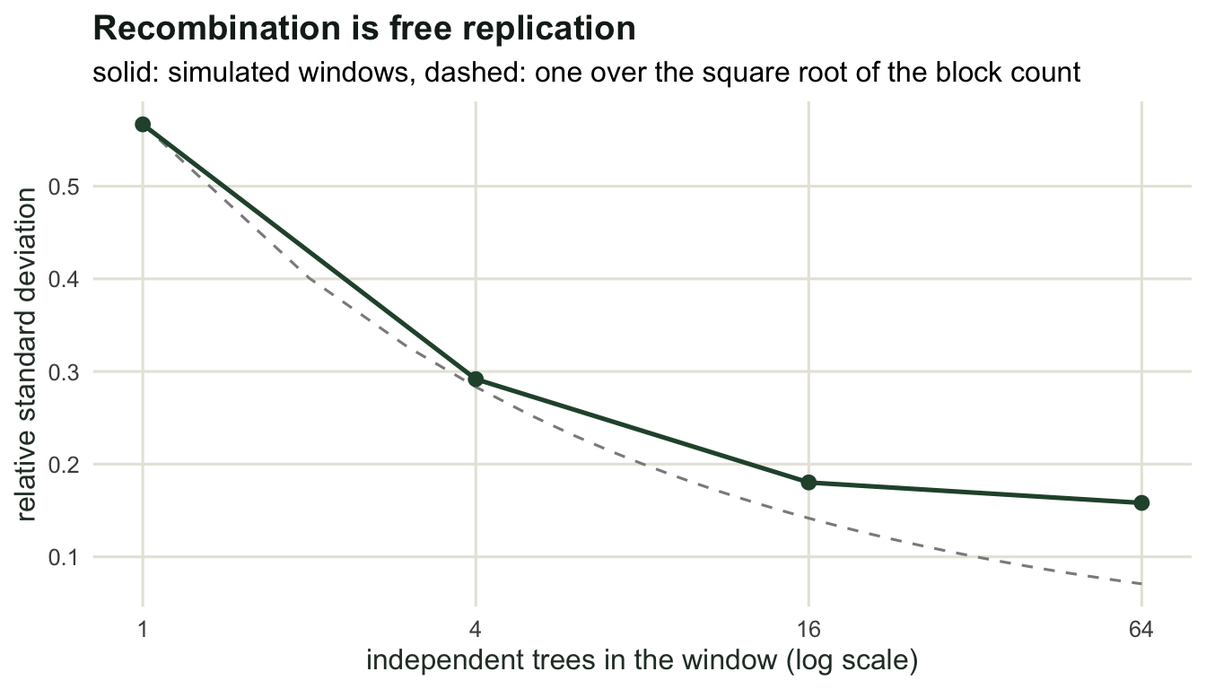

Figure 1: Relative standard deviation of the diversity estimate against the number of independent trees in a window of fixed total mutational opportunity.

Check 3: does demography really mimic selection?

The standard warning is that demographic change and selection both distort the frequency spectrum, so a significant Tajima’s D proves nothing. That warning is right in spirit and worth measuring rather than repeating, because the size of the problem depends on which demography.

Three histories: a completed sweep, which leaves a star-shaped genealogy; exponential growth at three rates; and a bottleneck.

set.seed(488)
star_d <- function(n, theta, height) {
  br <- cbind(descendants = rep(1L, n), length = rep(height, n))
  stats_sfs(sfs_from_tree(br, n, theta), n)
}

sweep_vals <- t(replicate(1200, star_d(n, theta * 3, 0.15)))
lo <- quantile(sweep_vals[, "D"], 0.05, na.rm = TRUE)
hi <- quantile(sweep_vals[, "D"], 0.95, na.rm = TRUE)
cat("sweep-like star tree: mean D", round(mean(sweep_vals[, "D"], na.rm = TRUE), 3),
    " 5th and 95th percentile", round(lo, 3), round(hi, 3), "\n")

sweep-like star tree: mean D -2.471  5th and 95th percentile -2.534 -2.381 

grow <- function(alpha) function(t) exp(-alpha * t)
for (alpha in c(5, 20, 50)) {
  gv <- t(replicate(600, stats_sfs(
    sfs_from_tree(coal_branches(n, size_fun = grow(alpha)), n, theta), n)))
  cat("growth alpha", alpha, ": mean D",
      round(mean(gv[, "D"], na.rm = TRUE), 3),
      " fraction below -2", round(mean(gv[, "D"] < -2, na.rm = TRUE), 4),
      " fraction inside the sweep interval",
      round(mean(gv[, "D"] >= lo & gv[, "D"] <= hi, na.rm = TRUE), 4), "\n")
}

growth alpha 5 : mean D -0.711  fraction below -2 0.0084  fraction inside the sweep interval 0 
growth alpha 20 : mean D -0.932  fraction below -2 0.0059  fraction inside the sweep interval 0 
growth alpha 50 : mean D -1.069  fraction below -2 0  fraction inside the sweep interval 0 

bott <- function(depth, t0, t1) function(t) if (t > t0 && t < t1) depth else 1
bv <- t(replicate(600, stats_sfs(
  sfs_from_tree(coal_branches(n, size_fun = bott(0.1, 0.05, 0.2)), n, theta),
  n)))
nv <- t(replicate(600, stats_sfs(sfs_from_tree(coal_branches(n), n, theta), n)))
cat("bottleneck: mean D", round(mean(bv[, "D"], na.rm = TRUE), 3),
    " fraction below -2", round(mean(bv[, "D"] < -2, na.rm = TRUE), 4),
    " fraction above 2", round(mean(bv[, "D"] > 2, na.rm = TRUE), 4), "\n")

bottleneck: mean D -0.416  fraction below -2 0.0223  fraction above 2 0.0372 

cat("constant size: mean D", round(mean(nv[, "D"], na.rm = TRUE), 3),
    " fraction below -2", round(mean(nv[, "D"] < -2, na.rm = TRUE), 4),
    " fraction above 2", round(mean(nv[, "D"] > 2, na.rm = TRUE), 4), "\n")

constant size: mean D -0.105  fraction below -2 0.0067  fraction above 2 0.0117 

The measurement refines the warning in three ways.

A completed sweep drives D to the lower bound the statistic can reach for this sample size: mean -2.471 with a 5th to 95th percentile of -2.534 to -2.381, an extremely tight distribution because a star tree produces nothing but singletons. So magnitude does carry information, and an extreme D is not something demography produces easily.

Exponential growth shifts the mean, from -0.711 at a growth rate of 5 to -1.069 at 50, but it barely populates the tail beyond the conventional cutoff (0.84 percent, 0.59 percent and 0 percent below -2), and not one growth locus in any of the three runs landed inside the sweep interval. Growth mostly moves the centre of the distribution, not its extreme.

The bottleneck is the dangerous one. Its mean D is only mildly negative (-0.416), but the fractions in both tails roughly triple against the neutral reference measured in the same run: 2.23 percent below -2 and 3.72 percent above +2, against 0.67 and 1.17 percent under constant size. That is the case where a per-locus cutoff calibrated on a constant-size null produces spurious outliers in both directions, and no amount of extra sequencing removes it, because the excess comes from the demography rather than from noise.

The check therefore has a definite recipe. Calibrate the outlier threshold against a demographic null fitted to the data, not against the constant-size expectation, and use the genome-wide distribution as the reference. Report the shift of the whole distribution as evidence about history, and only the tails against a matched null as evidence about selection.

gv50 <- t(replicate(600, stats_sfs(
  sfs_from_tree(coal_branches(n, size_fun = grow(50)), n, theta), n)))
conf_df <- rbind(
  data.frame(D = sweep_vals[, "D"], history = "completed sweep"),
  data.frame(D = gv50[, "D"], history = "growth, alpha 50"),
  data.frame(D = bv[, "D"], history = "bottleneck"),
  data.frame(D = nv[, "D"], history = "constant size"))

ggplot(subset(conf_df, !is.na(D)), aes(D, colour = history)) +
  geom_vline(xintercept = c(-2, 2), linetype = "dashed",
             colour = te_pal$line) +
  geom_density(linewidth = 0.9) +
  scale_colour_manual(values = c(`completed sweep` = te_pal$clay,
                                 `growth, alpha 50` = te_pal$gold,
                                 bottleneck = te_pal$sage,
                                 `constant size` = te_pal$ink),
                      name = NULL) +
  labs(title = "Not every demography reaches the tail",
       subtitle = "600 to 1200 loci per history, 20 sequences, theta 5",
       x = "Tajima's D", y = "density") +
  theme_te()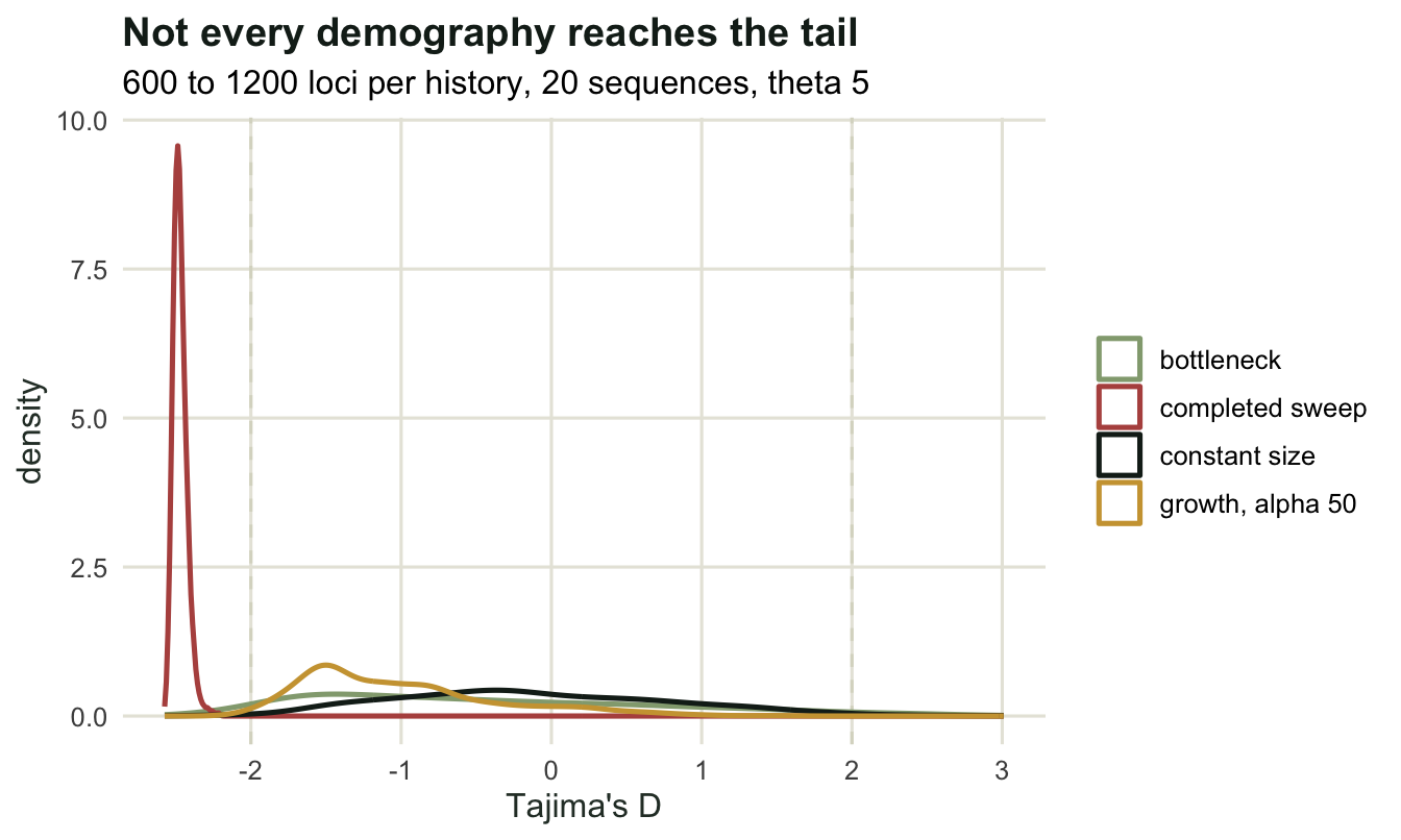

Figure 2: Tajima’s D under a completed sweep, strong growth, a bottleneck and constant size, with the conventional cutoffs marked.

Check 4: sequences or loci?

The last check is the design question in coalescent currency. Total branch length grows with the logarithm of the sample size, so extra sequences add mutations slowly, while extra loci add independent trees.

set.seed(489)
design2 <- function(n_seq, n_loci, theta_l = 5, reps = 400) {
  a1 <- sum(1 / seq_len(n_seq - 1))
  out <- replicate(reps, {
    s <- replicate(n_loci, sum(sfs_from_tree(coal_branches(n_seq), n_seq,
                                             theta_l)))
    mean(s) / a1
  })
  c(sequences = n_seq, loci = n_loci, mean = mean(out), sd = sd(out),
    relative_sd = sd(out) / mean(out))
}

print(round(rbind(design2(10, 10), design2(40, 10), design2(10, 40)), 4))

     sequences loci   mean     sd relative_sd
[1,]        10   10 4.9442 0.8379      0.1695
[2,]        40   10 4.9394 0.5470      0.1107
[3,]        10   40 5.0073 0.4448      0.0888

Starting from ten sequences at ten loci (relative standard deviation 0.1695), quadrupling the sequences improves it to 0.1107 and quadrupling the loci to 0.0888. The loci win, and they win by roughly the factor the square-root rule predicts while the sequences do not, because each locus is a fresh draw of ancestry and each extra sequence is another twig on a tree that already exists. Sampling more individuals is still worth doing when the question is about individuals (relatedness, inbreeding, structure), but for a parameter of the population’s history, independent loci are what buy precision.

The honest limit

Three assumptions sit under everything above, and each one fails somewhere.

The coalescent used here is panmictic, constant-size and neutral by default, and every departure was implemented as a modification of the same machinery. That is convenient, and it hides how strongly the conclusions depend on the model class. Nothing in a frequency spectrum tells you it was generated by a structured population rather than a growing one; the two produce different spectra, but a spectrum consistent with one is often consistent with some parameterisation of the other. Fitting one demographic model and testing selection against it is a coherent procedure only if the model class is broad enough to contain the truth, and it usually is not.

The mutation model is simple: one mutation per site, no back mutation, no rate heterogeneity. Sequencing error inflates singletons, which drags D down; a filter that removes singletons drags it up. Both are decisions made before the analysis and both move the statistic more than most biological effects.

The timescale is in units of 2N generations, which means every result is about Ne and about mutation rate as a product. A coalescent analysis can say the tree is twice as deep in one population as another; converting that into years needs a mutation rate and a generation time from outside the data, and the uncertainty in those is often larger than the uncertainty in the genetics.

Where to go next

That closes the coalescent cluster, and with it the population genetics arc: expectations for one locus, differentiation among populations, drift and gene flow, effective size and its estimators, and now the backward view with its diversity statistics and their diagnostics. The obvious continuation is where these methods meet geography: landscape genetics, where the resistance of the terrain between populations becomes the explanatory variable, and where the statistical trap is the one the Mantel test tutorial already sets up.

References

Hudson RR 2002 Bioinformatics 18(2):337-338 (10.1093/bioinformatics/18.2.337)

Wall JD 1999 Molecular Biology and Evolution 16(6):814-822 (10.1093/oxfordjournals.molbev.a026164)

Nielsen R 2005 Annual Review of Genetics 39:197-218 (10.1146/annurev.genet.39.073003.112420)

Beaumont MA, Zhang W, Balding DJ 2002 Genetics 162(4):2025-2035 (10.1093/genetics/162.4.2025)

Related tutorials

• The coalescent and gene trees
• Nucleotide diversity and Watterson theta
• Tajima’s D and the frequency spectrum
• Checking an effective size estimate