Nucleotide diversity and Watterson theta

Put mutations on coalescent trees in R, compare the two classical estimators of theta, and measure why many short loci beat one long sequence of the same size.

A gene tree is not observable. What a sequencing run returns is a set of variable sites, and those sites are mutations that happened to fall on the branches of the unobserved tree. Since mutations arrive at a constant rate along branches, the number of them is proportional to total branch length, and the pattern they leave depends on which branches they landed on.

Two summaries of that pattern have been in use since the 1970s: the average number of differences between pairs of sequences, and the number of segregating sites scaled by a combinatorial constant. Both estimate the same parameter under neutrality, and their disagreement is the subject of the next tutorial. This one builds them and measures which is sharper.

Mutations on a tree

The scaled mutation parameter is theta = 4Nu, and with time in units of 2N generations, mutations fall on a branch of length t at rate theta/2. Simulating a locus therefore takes two steps: draw a tree, then draw Poisson mutations on each branch. To know what a mutation looks like in the sample, each branch is tagged with the number of sampled copies that descend from it: a mutation on a branch with i descendants produces a variant carried by i of the n sequences.

library(ggplot2)

te_pal <- list(forest = "#275139", green = "#2f8f63", sage = "#93a87f",
               clay = "#b5534e", gold = "#cda23f", line = "#dad9ca",
               ink = "#16241d")

theme_te <- function() {
  theme_minimal(base_size = 12) +
    theme(panel.grid.minor = element_blank(),
          panel.grid.major = element_line(colour = "#e7e6dc"),
          plot.background = element_rect(fill = "white", colour = NA),
          panel.background = element_rect(fill = "white", colour = NA),
          plot.title = element_text(face = "bold", colour = te_pal$ink),
          axis.title = element_text(colour = "#2c3a31"))
}

coal_branches <- function(n) {
  counts <- rep(1L, n)
  lens <- rep(0, n)
  out <- NULL
  while (length(counts) > 1) {
    k <- length(counts)
    lens <- lens + rexp(1, rate = k * (k - 1) / 2)
    pick <- sample(k, 2)
    out <- rbind(out, cbind(counts[pick], lens[pick]))
    counts <- c(counts[-pick], sum(counts[pick]))
    lens <- c(lens[-pick], 0)
  }
  colnames(out) <- c("descendants", "length")
  out
}

sfs_from_tree <- function(br, n, theta) {
  muts <- rpois(nrow(br), theta / 2 * br[, "length"])
  tabulate(rep(br[, "descendants"], muts), nbins = n - 1)
}

stats_sfs <- function(sfs, n) {
  i <- seq_along(sfs)
  a1 <- sum(1 / seq_len(n - 1))
  s_tot <- sum(sfs)
  c(S = s_tot,
    pi = sum(sfs * 2 * i * (n - i)) / (n * (n - 1)),
    theta_w = s_tot / a1)
}

The site frequency spectrum, sfs, is the whole summary: element i counts variants carried by i sequences. Nucleotide diversity pi is the mean pairwise difference, which can be read straight off the spectrum because a variant at count i differs between i(n - i) of the n(n-1)/2 pairs. Watterson’s estimator divides the total number of segregating sites by a1 = sum(1/k), which is the expected total branch length in units of 2N.

Two unbiased estimators, one of them sharper

Simulate 4000 independent loci from a population with theta = 5, sampling 20 sequences each.

set.seed(481)
n <- 20
theta <- 5
loci <- 4000

est <- t(replicate(loci, stats_sfs(sfs_from_tree(coal_branches(n), n, theta),
                                   n)))

cat("mean pi", round(mean(est[, "pi"]), 4),
    " sd", round(sd(est[, "pi"]), 4), "\n")

mean pi 4.9212  sd 2.7778 

cat("mean Watterson theta", round(mean(est[, "theta_w"]), 4),
    " sd", round(sd(est[, "theta_w"]), 4), "\n")

mean Watterson theta 4.9457  sd 2.0985 

cat("mean segregating sites", round(mean(est[, "S"]), 3),
    " expected theta * a1", round(theta * sum(1 / seq_len(n - 1)), 3), "\n")

mean segregating sites 17.546  expected theta * a1 17.739 

cat("correlation between the two estimators",
    round(cor(est[, "pi"], est[, "theta_w"]), 4), "\n")

correlation between the two estimators 0.8669 

Both estimators land on the truth: 4.9212 and 4.9457 against a true 5, and the mean number of segregating sites is 17.546 against an expected 17.739. The interesting column is the spread. Watterson’s estimator has a standard deviation of 2.0985 and nucleotide diversity 2.7778, so the segregating-sites estimator is about a third sharper on a single locus.

The reason is which part of the tree each one weights. Every mutation counts once towards S, wherever it fell, so Watterson’s estimator uses the whole tree. Nucleotide diversity weights a variant by i(n - i), which peaks for variants carried by half the sample and gives almost nothing to singletons, so it is dominated by the deep branches: precisely the part of the tree that the previous tutorial showed to be a single long, highly variable interval. Weighting the noisiest part of the tree most heavily costs precision.

That does not make pi the wrong choice. It is the quantity with a direct interpretation (expected differences between two random sequences), it is comparable across studies with different sample sizes, and it is far less sensitive to sequencing error, which manufactures singletons and inflates S. The estimators also agree strongly with each other, correlation 0.8669, because both are functions of the same tree.

est_df <- rbind(
  data.frame(value = est[, "pi"], estimator = "pi (pairwise differences)"),
  data.frame(value = est[, "theta_w"], estimator = "Watterson (segregating sites)"))

ggplot(est_df, aes(value, colour = estimator)) +
  geom_density(linewidth = 0.9) +
  geom_vline(xintercept = theta, linetype = "dashed", colour = "grey40") +
  coord_cartesian(xlim = c(0, 15)) +
  scale_colour_manual(values = c(`pi (pairwise differences)` = te_pal$clay,
                                 `Watterson (segregating sites)` = te_pal$forest),
                      name = NULL) +
  labs(title = "Same expectation, different precision",
       subtitle = "4000 loci, true theta 5, 20 sequences each",
       x = "estimate of theta", y = "density") +
  theme_te()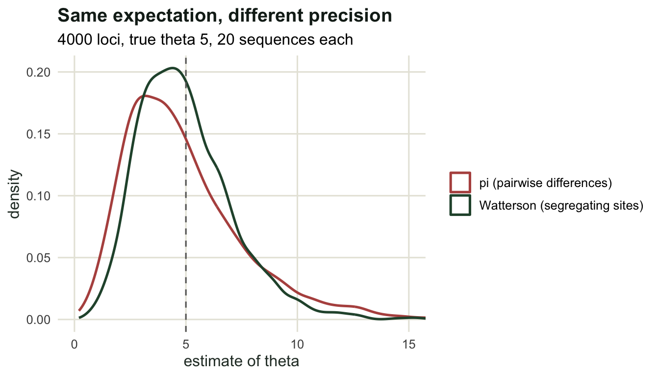

Figure 1: Distributions of the two estimators across 4000 independent loci simulated with a true theta of 5, 20 sequences per locus.

The shape the neutral model predicts

The spectrum itself has an expectation worth knowing by heart: under neutrality and constant size, the expected number of variants carried by i copies is theta/i. Singletons are the largest class, doubletons half that, and so on.

set.seed(483)
sfs_mean <- rowMeans(replicate(3000, sfs_from_tree(coal_branches(n), n, theta)))
print(round(rbind(simulated = sfs_mean[1:6],
                  `theta / i` = theta / (1:6)), 4))

           [,1]   [,2]   [,3]  [,4]  [,5]   [,6]
simulated 5.032 2.5523 1.6587 1.266 1.021 0.8777
theta / i 5.000 2.5000 1.6667 1.250 1.000 0.8333

Simulated 5.032, 2.5523, 1.6587, 1.266, 1.021, 0.8777 against predicted 5, 2.5, 1.6667, 1.25, 1, 0.8333. That 1/i shape is the reference against which every departure gets measured, and departures are what the next tutorial is about.

spec_df <- data.frame(i = seq_along(sfs_mean), simulated = sfs_mean,
                      predicted = theta / seq_along(sfs_mean))

ggplot(spec_df, aes(i, simulated)) +
  geom_col(fill = te_pal$sage, colour = "white") +
  geom_point(aes(y = predicted), colour = te_pal$clay, size = 2) +
  labs(title = "The neutral spectrum falls as one over the count",
       subtitle = "bars: 3000 simulated loci; points: theta / i",
       x = "variant carried by i of 20 sequences",
       y = "mean number of variants") +
  theme_te()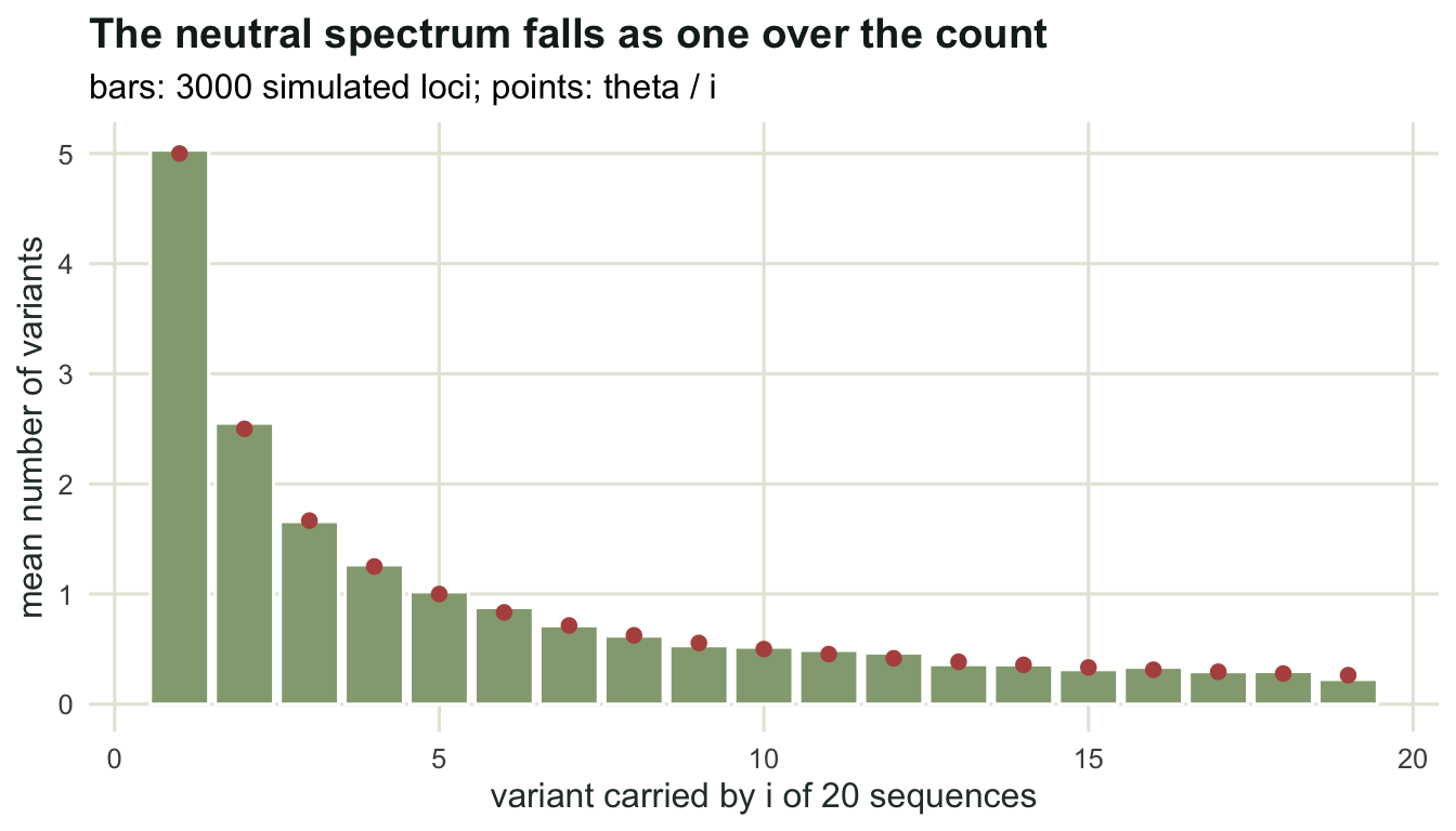

Figure 2: Mean site frequency spectrum from 3000 neutral loci against the theta/i expectation.

Many short loci beat one long sequence

Here is the design question in its coalescent form. Suppose the sequencing budget is fixed, so the total mutational opportunity is fixed: a total theta of 20 can be one locus with theta = 20, four loci with 5 each, or twenty loci with 1 each. Which arrangement estimates theta most precisely?

set.seed(482)
design_var <- function(n_loci, theta_per_locus, reps = 400) {
  out <- replicate(reps, {
    tot <- replicate(n_loci, sum(sfs_from_tree(coal_branches(n), n,
                                               theta_per_locus)))
    sum(tot) / (n_loci * sum(1 / seq_len(n - 1)))
  })
  c(loci = n_loci, theta_per_locus = theta_per_locus,
    mean = mean(out), sd = sd(out), relative_sd = sd(out) / mean(out))
}

print(round(rbind(design_var(1, 20), design_var(4, 5), design_var(20, 1)), 4))

     loci theta_per_locus    mean     sd relative_sd
[1,]    1              20 19.8302 7.7334      0.3900
[2,]    4               5  5.0425 1.0744      0.2131
[3,]   20               1  0.9836 0.1456      0.1481

One locus carrying all the variation gives a relative standard deviation of 0.39. The same total sequence split into four loci gives 0.2131, and into twenty loci 0.148. Nothing about the mutation process changed; what changed is the number of independent gene trees. Sites in one non-recombining locus all sit on the same tree, so they are not independent observations of the demographic history, they are repeated observations of one realisation of it, and the tree’s own variance sets a floor that no extra sequence length can break.

This is the same conclusion the effective-size tutorials reached from the other direction, and it is worth stating as a rule: for questions about demography, spend the budget on independent regions, not on sequencing one region deeply. Recombination helps, because a recombining region is a mosaic of trees rather than a single one, which is one reason genome-scale data behaves better than the classical single-locus theory suggests.

One naming caution. This blog has a tutorial on the Ewens sampling formula and Watterson’s exact test for neutrality, and that one is about species abundances in an ecological community, not about sequences. The mathematics is shared, the same names attach to both, and the objects are different: species in a sample there, gene copies in a sample here. Do not read a theta from one context into the other.

Where to go next

Two estimators of the same parameter, weighting different parts of the tree, and disagreeing whenever the tree is not the shape the neutral constant-size model predicts. That difference, standardised, is Tajima’s D, and the next tutorial measures what it detects, what it confuses, and how often it is wrong.

References

Watterson GA 1975 Theoretical Population Biology 7(2):256-276 (10.1016/0040-5809(75)90020-9)

Nei M, Li WH 1979 Proceedings of the National Academy of Sciences 76(10):5269-5273 (10.1073/pnas.76.10.5269)

Tajima F 1983 Genetics 105(2):437-460 (10.1093/genetics/105.2.437)

Fu YX, Li WH 1993 Genetics 133(3):693-709 (10.1093/genetics/133.3.693)

Related tutorials

• The coalescent and gene trees
• Tajima’s D and the frequency spectrum
• Checking a coalescent analysis
• Effective population size