library(ggplot2)
library(patchwork)

te_paper  <- "#f5f4ee"
te_ink    <- "#16241d"
te_body   <- "#2c3a31"
te_forest <- "#275139"
te_rust   <- "#b5534e"
te_gold   <- "#c9b458"
te_line   <- "#dad9ca"

theme_datasheet <- function() {
  theme_minimal(base_size = 12) +
    theme(plot.background  = element_rect(fill = te_paper, colour = NA),
          panel.background = element_rect(fill = te_paper, colour = NA),
          panel.grid.major = element_line(colour = te_line, linewidth = 0.3),
          panel.grid.minor = element_blank(),
          text             = element_text(colour = te_body),
          plot.title       = element_text(colour = te_ink, face = "bold"),
          plot.subtitle    = element_text(colour = te_body),
          axis.text        = element_text(colour = te_body))
}Spike tests on logger data delete real peaks
R
data cleaning
monitoring
time series
simulation
ecology tutorial
Spike tests on logger data delete storm surges that span few readings. Running-median and three-point tests, geometry and simulation by logging interval, in R.
A temperature logger sits on the bed of an urban stream for a summer. Every so often a thunderstorm sends warm runoff off the roads and car parks, and the water warms by a few degrees for an hour or two before the surge passes downstream. Nelson and Palmer report rainstorm surges of this kind in urbanised streams that averaged about three and a half degrees and died away in about three hours. Those surges are the reason the logger is there: they are the thermal events that stress trout and invertebrates, and a summary of hours above a stressful temperature is built from them.
The same record also holds values that are simply wrong. A logger touched during a download, a loose connector, a burst of electrical noise or a sensor briefly out of the water all leave single readings that sit far from their neighbours. A common automated tool for them is a spike test: compare each reading with its neighbours, for instance their mean or the running median of the readings around it, and flag it when the difference passes a threshold. Campbell and colleagues argue that sensor data streams have outgrown manual checking and need automated quality control that keeps track of every change. Horsburgh and colleagues describe open software that applies such edits in a traceable, reproducible way. Leigh and colleagues compare automated anomaly detectors on river sensor records, find that regression-based methods classify sudden isolated spikes well, and recommend combining methods to keep false positives down. A false positive here is a real reading flagged as a fault. This post measures how often a spike test produces one. Most of the answer is set by a design decision made before the logger went into the water, how often it records, and a smaller part by which neighbours the test compares with.
The mechanism is not subtle. An artefact is one reading wide at any logging interval. A surge that lasts an hour and a half spans eighteen readings at a five-minute interval and one or two readings at an hourly interval. A rule that looks at neighbours can tell those apart only while the surge is wider than the artefact, and the logging interval decides that. Most of this is plain geometry, which a later section writes down as a formula and checks against the simulation; the simulation is needed for the rest: what the same thresholds do to artefact catch, how a threshold scaled to the data misleads, and what the lost crests do to the summaries.
Other posts on this site price checks and deletions of a different kind. Data entry errors and what your checks catch scores range rules and double entry on a keyed field table, where each value stands alone and there is no time axis to borrow neighbours from. Deleting outliers before the test measures what removing large residuals does to the error rate of a regression. Where the night-time flux comes from examines a friction velocity screen, which discards whole half hours because of the conditions, not because a reading looks odd, and Gap filling a flux time series treats instrument flags as a cause of missing data that is already known. Here the detector itself is under test, on a series, and the quantities that set its performance are the width of a real event measured in logging intervals and its height against the threshold.
The post simulates 120 days of stream temperature with a diel cycle, slow noise, storm surges and one-reading artefacts, logs it at four intervals and scores five spike rules: four built on a five-reading running median and the three-point test from the real-time checks of the Argo quality control manual. It then sweeps the threshold, sweeps the surge width and the surge height against the threshold, and follows the damage into two summaries an ecologist would report: the record maximum and the hours above 20 degrees.
A logger record with surges and glitches
n_day    <- 120
base_min <- 5
n_base   <- n_day * 24 * 60 / base_min
t_min    <- (seq_len(n_base) - 1) * base_min

diel_amp  <- 3
ar_phi    <- 0.98
ar_sd     <- 0.08
ev_per_day <- 1 / 3
fwhm_sdlog <- 0.6
amp_lo <- 2
amp_hi <- 5
art_share <- 0.005
art_lo <- 2
art_hi <- 6
step_set <- c(1, 3, 6, 12)
iv_set   <- step_set * base_min
k_set    <- c(4, 6)
thr_phys <- 1.5
hot_line <- 20

sim_series <- function(fwhm_med) {
  diel  <- diel_amp * sin(2 * pi * (t_min / 60 - 9) / 24)
  ar_part <- as.numeric(stats::filter(rnorm(n_base, 0, ar_sd), ar_phi,
                                      method = "recursive"))
  n_ev  <- rpois(1, ev_per_day * n_day)
  ctr   <- runif(n_ev, 0, max(t_min))
  fwhm  <- rlnorm(n_ev, log(fwhm_med), fwhm_sdlog)
  amp   <- runif(n_ev, amp_lo, amp_hi)
  pulse <- numeric(n_base)
  for (i in seq_len(n_ev)) {
    s_g <- fwhm[i] / (2 * sqrt(2 * log(2)))
    w   <- which(abs(t_min - ctr[i]) < 5 * s_g)
    pulse[w] <- pulse[w] + amp[i] * exp(-0.5 * ((t_min[w] - ctr[i]) / s_g)^2)
  }
  list(x = 15 + diel + ar_part + pulse, base = 15 + diel + ar_part,
       ctr = ctr, fwhm = fwhm, amp = amp)
}

log_series <- function(sr, step, a_lo = art_lo, a_hi = art_hi) {
  idx  <- seq(1, n_base, by = step)
  x_ok <- sr$x[idx]
  m_n  <- length(x_ok)
  art  <- sample(m_n, round(art_share * m_n))
  x_log <- x_ok
  x_log[art] <- x_log[art] +
    sample(c(-1, 1), length(art), TRUE) * runif(length(art), a_lo, a_hi)
  med5  <- stats::runmed(x_log, 5, endrule = "keep")
  dev5  <- abs(x_log - med5)
  nb_dev <- pmax(c(0, dev5[-m_n]), c(dev5[-1], 0))
  dev0   <- abs(x_ok - stats::runmed(x_ok, 5, endrule = "keep"))
  nb_dev0 <- pmax(c(0, dev0[-m_n]), c(dev0[-1], 0))
  v_prev <- c(x_log[1], x_log[-m_n])
  v_next <- c(x_log[-1], x_log[m_n])
  spk3   <- abs(x_log - (v_prev + v_next) / 2) - abs((v_next - v_prev) / 2)
  pk <- pmin(pmax(round(sr$ctr / (step * base_min)) + 1, 1), m_n)
  on_art <- pk %in% art
  list(x_ok = x_ok, x_log = x_log, base_log = sr$base[idx], art = art,
       dev5 = dev5, nb_dev = nb_dev, nb_dev0 = nb_dev0, spk3 = spk3,
       mad_diff = mad(diff(x_log)), pk = pk[!on_art], amp = sr$amp[!on_art],
       ratio = sr$fwhm[!on_art] / (step * base_min), n_on_art = sum(on_art))
}
The simulated record is 120 days at a 5-minute resolution. Water temperature is 15 degrees plus a diel sine wave of amplitude 3 degrees and a first order autoregressive component with lag one correlation 0.98 per five minutes. Storm surges arrive as a Poisson process, 0.33 per day on average, each a Gaussian bump centred at a continuous time, so that its peak can fall anywhere between two readings. Surge height is uniform between 2 and 5 degrees, and surge width at half height is lognormal with a log standard deviation of 0.6 around a median that is a design constant: 90 minutes in the main runs, with 45 and 180 minutes added for the sweep.
The record is then logged by taking every first, third, sixth or twelfth reading, which gives intervals of 5, 15, 30 and 60 minutes, and artefacts are added to the logged values: 0.5 per cent of readings, each shifted up or down by between 2 and 6 degrees. The artefact sizes overlap the surge heights on purpose, so that size alone cannot separate them; a later section removes the overlap.
Four of the rules compare a reading with the running median of the five logged readings centred on it. The first version flags a reading when its distance from that median exceeds k times the median absolute deviation of the first differences of the whole logged series, with k of 4 or 6. The second version uses a fixed threshold in physical units, 1.5 degrees, at every interval. The third adds a duration condition to the second: a reading is flagged only if neither neighbour is itself more than half the threshold from its own running median, so that a feature two or more readings wide is spared. The fifth rule is the three-point spike test written in the Argo quality control manual (Wong and colleagues), where it is applied to neighbouring depths of a profile: the test value is |V2 - (V1 + V3)/2| - |(V3 - V1)/2|, with V2 the reading and V1 and V3 its two neighbours, and here it is flagged above the same 1.5 degrees. At a local maximum the test value equals the smaller of the two steps up to the reading, so a crest that falls between two readings scores low. All thresholds were fixed before the simulation ran, and the three-point rule was added after review, with the same seeds.
Two rates are scored. Artefact catch is the share of artefacts flagged. Peak deletion is the share of real surges whose logged peak reading, the reading nearest the surge centre, is flagged; surges whose peak reading was itself hit by an artefact are left out of that denominator.
set.seed(3107)
demo <- sim_series(90)
demo_5  <- log_series(demo, 1)
demo_60 <- log_series(demo, 12)
flag_60 <- demo_60$dev5 > thr_phys
pk_60   <- pmin(pmax(round(demo$ctr / 60) + 1, 1), length(flag_60))
hit_ev  <- which(flag_60[pk_60])
hit_ev  <- hit_ev[which.max(demo$amp[hit_ev])]
ctr_h   <- demo$ctr[hit_ev] / 60
win_h   <- c(floor(ctr_h) - 12, floor(ctr_h) + 12)
hit_amp <- demo$amp[hit_ev]
hit_fw  <- demo$fwhm[hit_ev]

panel_df <- function(lg, step, lab) {
  hrs <- (seq_along(lg$x_log) - 1) * step * base_min / 60
  kind <- rep("kept", length(hrs))
  kind[lg$dev5 > thr_phys] <- "flagged, real signal"
  kind[intersect(lg$art, which(lg$dev5 > thr_phys))] <- "flagged, artefact"
  kind[setdiff(lg$art, which(lg$dev5 > thr_phys))] <- "missed artefact"
  keep <- hrs >= win_h[1] & hrs <= win_h[2]
  data.frame(hour = hrs[keep] - win_h[1], temp = lg$x_log[keep],
             kind = kind[keep], panel = lab)
}
win_df <- rbind(panel_df(demo_5, 1, "logged every 5 minutes"),
                panel_df(demo_60, 12, "logged every 60 minutes"))
win_df$panel <- factor(win_df$panel, levels = c("logged every 5 minutes",
                                                "logged every 60 minutes"))
kind_col <- c("kept" = te_line, "flagged, artefact" = te_forest,
              "flagged, real signal" = te_rust, "missed artefact" = te_gold)

ggplot(win_df, aes(hour, temp)) +
  geom_line(colour = te_body, linewidth = 0.4) +
  geom_point(data = win_df[win_df$kind != "kept", ], aes(colour = kind),
             size = 2.6) +
  scale_colour_manual(values = kind_col, name = NULL, drop = FALSE) +
  facet_wrap(~panel, ncol = 1) +
  labs(x = "hours into the window", y = "water temperature (degrees C)",
       title = "The same surge, two logging intervals",
       subtitle = "flag: sample more than 1.5 degrees from its 5-sample running median") +
  theme_datasheet() +
  theme(legend.position = "bottom")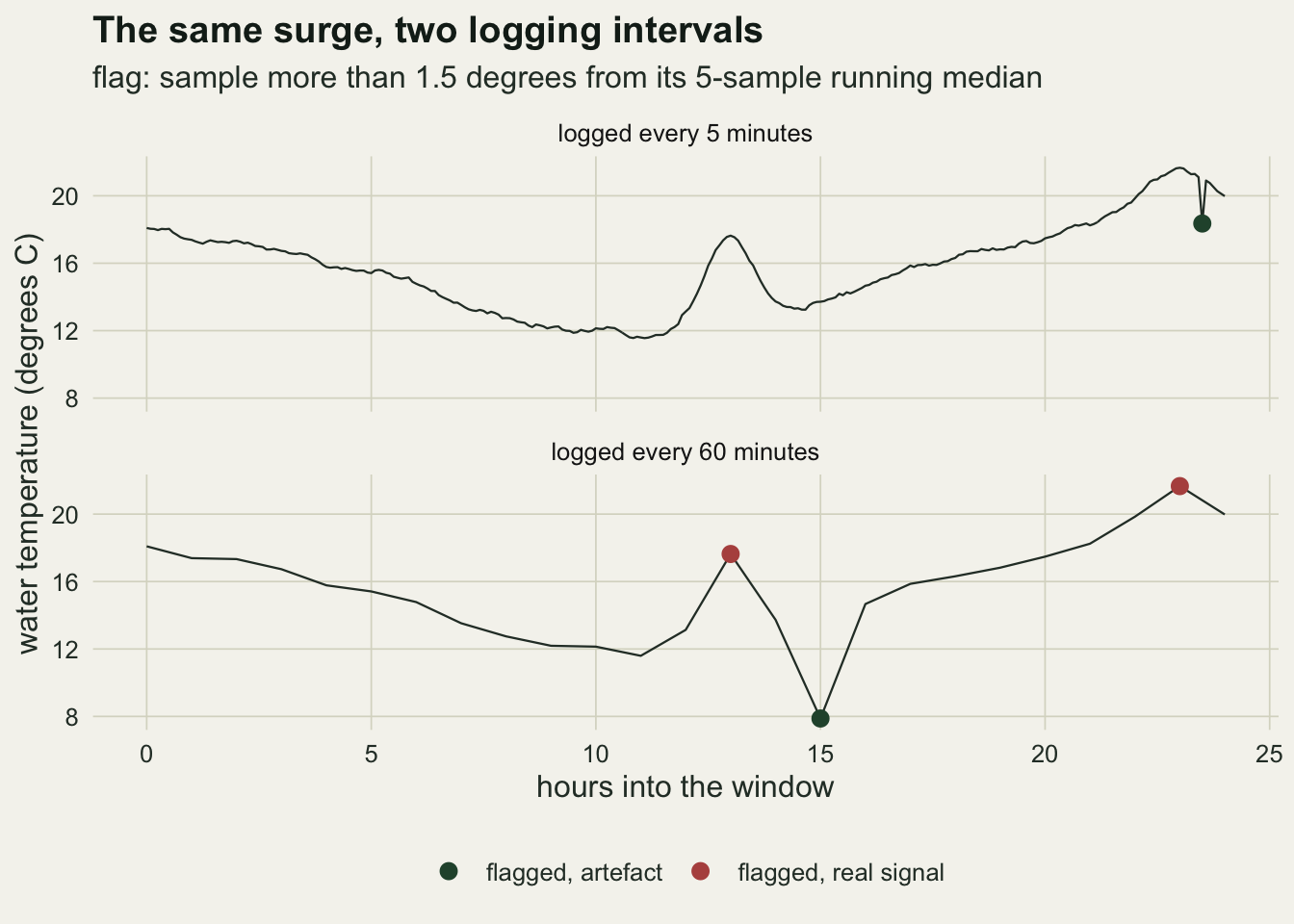
The figure above shows one day of one record, centred on the tallest surge whose hourly peak reading the fixed threshold flags. That surge is 5.0 degrees high and 79 minutes wide at half height. Choosing the window by its outcome is for illustration only; the rates below come from all surges.
Catching artefacts and deleting peaks, by interval
n_rep    <- 50
fwhm_set <- c(45, 90, 180)
thr_grid <- exp(seq(log(0.1), log(10), length.out = 80))

set.seed(20260910)
roc_list <- list(); ev_list <- list(); rate_list <- list(); qty_list <- list()
for (fw in fwhm_set) {
  for (r_i in seq_len(n_rep)) {
    sr <- sim_series(fw)
    for (step in step_set) {
      lg <- log_series(sr, step)
      roc_list[[length(roc_list) + 1]] <- data.frame(
        fwhm_med = fw, iv = step * base_min, thr = thr_grid,
        n_art = length(lg$art), n_pk = length(lg$pk),
        c_art = vapply(thr_grid, function(h) sum(lg$dev5[lg$art] > h), 0),
        c_pk  = vapply(thr_grid, function(h) sum(lg$dev5[lg$pk] > h), 0),
        c_art3 = vapply(thr_grid, function(h) sum(lg$spk3[lg$art] > h), 0),
        c_pk3  = vapply(thr_grid, function(h) sum(lg$spk3[lg$pk] > h), 0))
      ev_list[[length(ev_list) + 1]] <- data.frame(
        fwhm_med = fw, iv = step * base_min, ratio = lg$ratio, amp = lg$amp,
        dev_pk = lg$dev5[lg$pk], nb_pk = lg$nb_dev[lg$pk], spk_pk = lg$spk3[lg$pk],
        del_med = lg$dev5[lg$pk] > thr_phys,
        del_dur = lg$dev5[lg$pk] > thr_phys & lg$nb_dev[lg$pk] < thr_phys / 2,
        del_q3  = lg$spk3[lg$pk] > thr_phys)
      if (fw == 90) {
        f_mad4 <- lg$dev5 > k_set[1] * lg$mad_diff
        f_mad6 <- lg$dev5 > k_set[2] * lg$mad_diff
        f_phys <- lg$dev5 > thr_phys
        f_dur  <- f_phys & lg$nb_dev < thr_phys / 2
        f_q3   <- lg$spk3 > thr_phys
        a_fl   <- lg$art[f_phys[lg$art]]
        rate_list[[length(rate_list) + 1]] <- data.frame(
          iv = step * base_min,
          rule = c("MAD-scaled, k = 4", "MAD-scaled, k = 6",
                   "fixed 1.5 degrees", "fixed 1.5 degrees, duration-aware",
                   "three-point, 1.5 degrees"),
          c_art = c(sum(f_mad4[lg$art]), sum(f_mad6[lg$art]),
                    sum(f_phys[lg$art]), sum(f_dur[lg$art]), sum(f_q3[lg$art])),
          n_art = length(lg$art),
          c_pk = c(sum(f_mad4[lg$pk]), sum(f_mad6[lg$pk]),
                   sum(f_phys[lg$pk]), sum(f_dur[lg$pk]), sum(f_q3[lg$pk])),
          n_pk = length(lg$pk), mad_diff = lg$mad_diff,
          n_afl = length(a_fl),
          nb_with = sum(lg$nb_dev[a_fl] >= thr_phys / 2),
          nb_without = sum(lg$nb_dev0[a_fl] >= thr_phys / 2))
        hrs_per <- step * base_min / 60
        x_qc <- lg$x_log
        x_qc[f_phys] <- NA
        x_q3 <- lg$x_log
        x_q3[f_q3] <- NA
        qty_list[[length(qty_list) + 1]] <- data.frame(
          iv = step * base_min,
          max_ok = max(lg$x_ok), max_raw = max(lg$x_log),
          max_qc = max(x_qc, na.rm = TRUE),
          hot_ok = sum(lg$x_ok > hot_line) * hrs_per,
          hot_raw = sum(lg$x_log > hot_line) * hrs_per,
          hot_qc = sum(x_qc > hot_line, na.rm = TRUE) * hrs_per,
          max_q3 = max(x_q3, na.rm = TRUE),
          hot_q3 = sum(x_q3 > hot_line, na.rm = TRUE) * hrs_per,
          hot_base = sum(lg$base_log > hot_line) * hrs_per)
      }
    }
  }
}
roc_all  <- do.call(rbind, roc_list)
ev_all   <- do.call(rbind, ev_list)
rate_all <- do.call(rbind, rate_list)
qty_all  <- do.call(rbind, qty_list)

rate_tab <- aggregate(cbind(c_art, n_art, c_pk, n_pk, mad_diff, n_afl, nb_with,
                            nb_without) ~ rule + iv, rate_all, sum)
rate_tab$catch <- rate_tab$c_art / rate_tab$n_art
rate_tab$del   <- rate_tab$c_pk / rate_tab$n_pk
rate_tab$del_se <- sqrt(rate_tab$del * (1 - rate_tab$del) / rate_tab$n_pk)
rate_tab$catch_se <- sqrt(rate_tab$catch * (1 - rate_tab$catch) / rate_tab$n_art)
rate_tab$mad_diff <- rate_tab$mad_diff / n_rep

get_rate <- function(rl, ivv, what) rate_tab[rate_tab$rule == rl & rate_tab$iv == ivv, what]
r_m4 <- "MAD-scaled, k = 4"; r_m6 <- "MAD-scaled, k = 6"
r_ph <- "fixed 1.5 degrees"; r_du <- "fixed 1.5 degrees, duration-aware"
r_q3 <- "three-point, 1.5 degrees"
nb_share <- function(ivv, what) get_rate(r_ph, ivv, what) / get_rate(r_ph, ivv, "n_afl")
diel_slope_h <- 2 * pi * diel_amp / 24
mad_5  <- get_rate(r_m6, 5, "mad_diff")
mad_60 <- get_rate(r_m6, 60, "mad_diff")
n_art_60 <- get_rate(r_ph, 60, "n_art")
n_pk_60  <- get_rate(r_ph, 60, "n_pk")
n_pk_5   <- get_rate(r_ph, 5, "n_pk")
max_del_se <- max(rate_tab$del_se)
At a 5-minute interval every version works. The MAD-scaled test with k of 6 catches 1.000 of 8650 artefacts and deletes 0.014 of 1988 surge peaks; the fixed threshold catches 0.999 and deletes 0.0005.
At 30 minutes the MAD-scaled test with k of 4 still catches 0.983 of artefacts, and it now deletes 0.314 of real surge peaks. The fixed threshold catches 0.988 and deletes 0.346. At 60 minutes the fixed threshold holds its catch at 0.960 of 700 artefacts and deletes 0.538 of 1993 surge peaks. The three-point test at the same 1.5 degrees catches 0.984 and 0.956 of artefacts at 30 and 60 minutes and deletes 0.117 and 0.313 of surge peaks: 0.34 of the running-median damage at 30 minutes and 0.58 of it at 60. The deletion rate therefore belongs to a rule and an interval together, not to spike testing as such. The largest Monte Carlo standard error of any deletion rate in the figure is 0.011.
The MAD-scaled lines look better at 60 minutes because they catch fewer artefacts: k of 4 catches 0.597 of them and k of 6 fewer still. The median absolute deviation of the first differences rises from 0.098 degrees at 5 minutes to 0.793 degrees at 60 minutes, because at an hourly interval the first differences are dominated by the diel slope rather than by the noise. A threshold of six such units at 60 minutes is 4.76 degrees, and the test with k of 6 catches only 0.206 of artefacts while deleting 0.0035 of peaks. Its falling deletion curve is a falling threshold, not a better test. Read against a MAD-scaled rule alone, the non-monotone deletion curve would suggest that hourly logging is safer than half-hourly logging; the fixed threshold shows it is not.
The duration condition does what it was built to do at intermediate intervals: at 30 minutes it deletes 0.125 of peaks against 0.346 without it, for a catch of 0.946. At 60 minutes it still deletes 0.297 of peaks, and its catch falls to 0.684, because the artefact itself sits inside each neighbour’s running-median window. On a rising or falling stretch it shifts that median by one reading’s worth of slope, and the diel slope alone reaches 0.79 degrees per hour. Of the artefacts the fixed threshold flags at 60 minutes, 0.287 have a neighbour at least three quarters of a degree from its own median; computed on the same record without artefacts, that share is 0.033.
rate_tab$rule <- factor(rate_tab$rule, levels = c(r_m6, r_m4, r_ph, r_du, r_q3))
rule_col <- setNames(c(te_gold, te_ink, te_rust, te_forest, te_rust),
                     levels(rate_tab$rule))
rule_lty <- setNames(c("solid", "solid", "solid", "solid", "22"),
                     levels(rate_tab$rule))
p_catch <- ggplot(rate_tab, aes(iv, catch, colour = rule, linetype = rule)) +
  geom_line(linewidth = 0.9) + geom_point(size = 2.2) +
  scale_colour_manual(values = rule_col, name = NULL) +
  scale_linetype_manual(values = rule_lty, name = NULL) +
  scale_x_continuous(breaks = iv_set) +
  scale_y_continuous(limits = c(0, 1)) +
  labs(x = "logging interval (minutes)", y = "share of artefacts caught",
       title = "Artefacts caught") +
  theme_datasheet()
p_del <- ggplot(rate_tab, aes(iv, del, colour = rule, linetype = rule)) +
  geom_line(linewidth = 0.9) + geom_point(size = 2.2) +
  scale_colour_manual(values = rule_col, name = NULL) +
  scale_linetype_manual(values = rule_lty, name = NULL) +
  scale_x_continuous(breaks = iv_set) +
  scale_y_continuous(limits = c(0, 1)) +
  labs(x = "logging interval (minutes)", y = "share of real peaks deleted",
       title = "Real peaks deleted") +
  theme_datasheet()
(p_catch | p_del) + plot_layout(guides = "collect") +
  plot_annotation(theme = theme_datasheet()) &
  guides(colour = guide_legend(nrow = 3), linetype = guide_legend(nrow = 3)) &
  theme(legend.position = "bottom")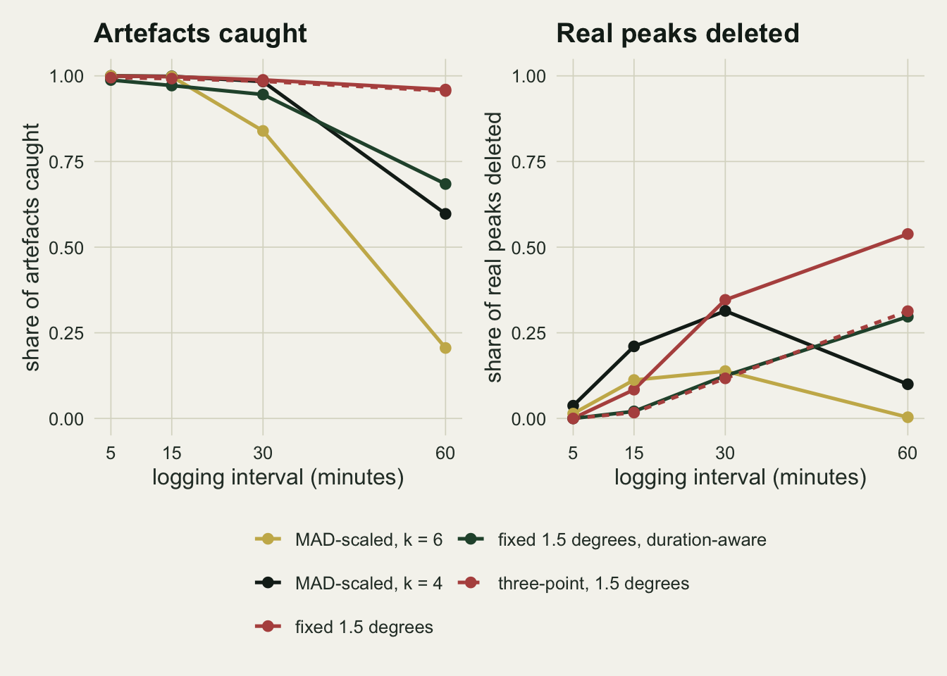
No threshold rescues the hourly record
roc_tab <- aggregate(cbind(c_art, n_art, c_pk, n_pk, c_art3, c_pk3) ~
                       fwhm_med + iv + thr, roc_all, sum)
roc_tab$catch  <- roc_tab$c_art / roc_tab$n_art
roc_tab$del    <- roc_tab$c_pk / roc_tab$n_pk
roc_tab$catch3 <- roc_tab$c_art3 / roc_tab$n_art
roc_tab$del3   <- roc_tab$c_pk3 / roc_tab$n_pk
at_catch <- function(fw, ivv, cc = "catch", dd = "del", target = 0.95) {
  s_r <- roc_tab[roc_tab$fwhm_med == fw & roc_tab$iv == ivv, ]
  s_r <- s_r[order(s_r$thr), ]
  j_r <- max(which(s_r[[cc]] >= target))
  c(thr = s_r$thr[j_r], catch = s_r[[cc]][j_r], del = s_r[[dd]][j_r])
}
op_tab <- expand.grid(fwhm_med = fwhm_set, iv = iv_set)
op_vals <- t(mapply(at_catch, op_tab$fwhm_med, op_tab$iv))
op_tab <- cbind(op_tab, op_vals)
op90 <- op_tab[op_tab$fwhm_med == 90, ]
del95 <- setNames(op90$del, op90$iv)
thr95 <- setNames(op90$thr, op90$iv)
op45  <- op_tab[op_tab$fwhm_med == 45, ]
op180 <- op_tab[op_tab$fwhm_med == 180, ]
op3_90 <- data.frame(iv = iv_set, t(vapply(iv_set, function(ivv)
  at_catch(90, ivv, "catch3", "del3"), numeric(3))))
del95_3 <- setNames(op3_90$del, op3_90$iv)

spare_at <- function(ivv, cc = "catch", dd = "del", max_del = 0.05) {
  s_r <- roc_tab[roc_tab$fwhm_med == 90 & roc_tab$iv == ivv, ]
  max(s_r[[cc]][s_r[[dd]] <= max_del])
}
spare_catch  <- setNames(vapply(iv_set, spare_at, 0), iv_set)
spare_catch3 <- setNames(vapply(iv_set, spare_at, 0, cc = "catch3", dd = "del3"),
                         iv_set)
A single threshold might simply be a poor choice for a coarse record. Sweeping the threshold of each test from 0.1 to 10 degrees, and pooling the 50 records at each interval, gives one trade-off curve per interval. The same records serve every threshold, so the curves differ only through the interval.
Take the threshold that first catches 95 per cent of artefacts. At 5 minutes that threshold is 2.07 degrees and it deletes 0.0005 of surge peaks. At 15 minutes it deletes 0.049, at 30 minutes 0.259, and at 60 minutes 0.515. Asking the question the other way round, and allowing the test to delete at most 5 per cent of real peaks, the best achievable artefact catch is 1.000 at 5 minutes, 0.967 at 15 minutes, 0.661 at 30 minutes and 0.470 at 60 minutes. For the three-point test the deletion at the 95 per cent catch threshold is 0.008 at 15 minutes, 0.084 at 30 minutes and 0.298 at 60 minutes, and the best catch at no more than 5 per cent deletion is 0.852 at 30 minutes and 0.541 at 60 minutes. The half-hourly record is partly rescued by the choice of test. On the hourly record neither test is both an artefact filter and a surge keeper.
The median surge width shifts the interval at which the trade-off opens. With surges half as wide, 45 minutes at the median, the 95 per cent catch threshold at 30 minutes deletes 0.518 of peaks; with surges twice as wide, 180 minutes, it deletes 0.048 at 30 minutes and 0.306 at 60 minutes.
roc90 <- roc_tab[roc_tab$fwhm_med == 90, ]
roc90$interval <- factor(paste(roc90$iv, "min"), levels = paste(iv_set, "min"))
op90$interval <- factor(paste(op90$iv, "min"), levels = paste(iv_set, "min"))
test_lab <- c("five-reading running median", "three-point test")
roc_long <- rbind(
  data.frame(roc90[, c("iv", "interval")], del = roc90$del, catch = roc90$catch,
             test = test_lab[1]),
  data.frame(roc90[, c("iv", "interval")], del = roc90$del3, catch = roc90$catch3,
             test = test_lab[2]))
roc_long$test <- factor(roc_long$test, levels = test_lab)
op_long <- rbind(
  data.frame(interval = op90$interval, del = op90$del, catch = op90$catch,
             test = test_lab[1]),
  data.frame(interval = op90$interval, del = op3_90$del, catch = op3_90$catch,
             test = test_lab[2]))
op_long$test <- factor(op_long$test, levels = test_lab)
ggplot(roc_long, aes(del, catch, colour = interval)) +
  geom_abline(slope = 1, intercept = 0, linetype = "dotted", colour = te_body) +
  geom_path(linewidth = 1) +
  geom_point(data = op_long, size = 3) +
  scale_colour_manual(values = c(te_forest, te_gold, te_rust, te_ink), name = NULL) +
  coord_equal(xlim = c(0, 1), ylim = c(0, 1)) +
  facet_wrap(~test) +
  labs(x = "share of real peaks deleted", y = "share of artefacts caught",
       title = "The trade-off opens as the interval grows",
       subtitle = "points: the threshold that first catches 95 per cent of artefacts") +
  theme_datasheet() +
  theme(legend.position = "bottom")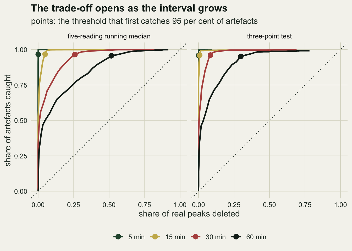
Width in readings is geometry
ev_all$bin_mid <- 2^(floor(log2(ev_all$ratio) * 2) / 2 + 0.25)

iv_coarse <- c(15, 30, 60)
band_rate <- function(lo, hi, what) {
  s_e <- ev_all[ev_all$ratio > lo & ev_all$ratio <= hi & ev_all$iv %in% iv_coarse, ]
  r_iv <- tapply(s_e[[what]], s_e$iv, mean)
  c(lo = min(r_iv), hi = max(r_iv), n = nrow(s_e))
}
b_12     <- band_rate(1, 2, "del_med")
b_23     <- band_rate(2, 3, "del_med")
b_34     <- band_rate(3, 4, "del_med")
b_4up    <- band_rate(4, Inf, "del_med")
b_01     <- band_rate(0, 1, "del_med")
b_12_dur <- band_rate(1, 2, "del_dur")
b_23_dur <- band_rate(2, 3, "del_dur")
b_01_dur <- band_rate(0, 1, "del_dur")
b_12_q3  <- band_rate(1, 2, "del_q3")
b_23_q3  <- band_rate(2, 3, "del_q3")
b_34_q3  <- band_rate(3, 4, "del_q3")
share_under3_60 <- mean(ev_all$ratio[ev_all$iv == 60 & ev_all$fwhm_med == 90] <= 3)
share_under3_15 <- mean(ev_all$ratio[ev_all$iv == 15 & ev_all$fwhm_med == 90] <= 3)

# noise-free geometry: a Gaussian crest of width w readings (at half height),
# sampled with its nearest reading `off` readings from the centre
cf_dev <- function(w, off, test) {
  v <- 2^(-4 * ((-2:2) + off)^2 / w^2)
  if (test == "median") v[3] - sort(v)[3] else v[3] - max(v[2], v[4])
}
off_grid <- seq(-0.5, 0.5, length.out = 41)
cf_del <- function(w, test, h) {
  d_o <- vapply(off_grid, function(o) cf_dev(w, o, test), 0)
  mean(pmin(pmax((amp_hi - h / d_o) / (amp_hi - amp_lo), 0), 1))
}
cf_edge <- function(test, h) {
  top <- function(w) max(vapply(off_grid, function(o) cf_dev(w, o, test), 0))
  uniroot(function(w) amp_hi * top(w) - h, c(1.2, 60))$root
}
cf_15 <- c(median = cf_del(1.5, "median", thr_phys), three = cf_del(1.5, "three", thr_phys))
cf_25 <- c(median = cf_del(2.5, "median", thr_phys), three = cf_del(2.5, "three", thr_phys))
cf_35 <- c(median = cf_del(3.5, "median", thr_phys), three = cf_del(3.5, "three", thr_phys))

# surge height against the threshold: the same surges scored at lower thresholds
h_sweep <- c(1.5, 0.75, 0.3)
hr_lab  <- sprintf("height / threshold %.1f to %.1f", amp_lo / h_sweep, amp_hi / h_sweep)
sw_list <- list()
for (j in seq_along(h_sweep)) {
  h <- h_sweep[j]
  sw_list[[j]] <- data.frame(bin_mid = ev_all$bin_mid, ratio = ev_all$ratio,
    iv = ev_all$iv, cls = hr_lab[j], h = h,
    median = ev_all$dev_pk > h, three = ev_all$spk_pk > h,
    dur = ev_all$dev_pk > h & ev_all$nb_pk < h / 2)
}
sw_all <- do.call(rbind, sw_list)
sw_band <- function(j, lo, hi, what) {
  s_e <- sw_all[sw_all$h == h_sweep[j] & sw_all$ratio > lo & sw_all$ratio <= hi &
                sw_all$iv %in% iv_coarse, ]
  mean(s_e[[what]])
}
edge_tab <- data.frame(h = h_sweep,
  med = vapply(h_sweep, function(h) cf_edge("median", h), 0),
  three = vapply(h_sweep, function(h) cf_edge("three", h), 0),
  sim_med_46 = vapply(1:3, function(j) sw_band(j, 4, 6, "median"), 0),
  sim_med_68 = vapply(1:3, function(j) sw_band(j, 6, 8, "median"), 0),
  sim_q3_46  = vapply(1:3, function(j) sw_band(j, 4, 6, "three"), 0),
  sim_med_12up = vapply(1:3, function(j) sw_band(j, 12, Inf, "median"), 0))
n_46 <- sum(ev_all$ratio > 4 & ev_all$ratio <= 6 & ev_all$iv %in% iv_coarse)
Take a Gaussian surge of height A whose width at half height is w readings, and suppose its crest falls exactly on a reading. The readings two to either side carry the height A times 2^(-4 p^2 / w^2), with p the distance in readings, so the running median of five is the value one reading away, and the crest stands A (1 - 2(-4/w2)) above it. For the three-point test the crest-centred value is the same; when the crest falls between two readings, the three-point value shrinks towards zero, while the running-median deviation grows for surges about two readings wide or more (for a surge one reading wide it shrinks too). The chunk above turns this into a noise-free deletion probability, averaging over where the crest falls between readings and over surge heights between 2 and 5 degrees, and finds the width beyond which even the tallest surge stays under the threshold. Nothing in that calculation depends on the interval or on the median surge width except through w, which is why surges from different intervals and median widths can be pooled on one axis: that collapse is built into the design, not discovered by it.
The simulation follows the geometry. Rates quote the 15, 30 and 60 minute records, where each band holds enough surges. For the running median at 1.5 degrees, the noise-free deletion is 0.99 at 1.5 readings, 0.58 at 2.5 and 0.049 at 3.5; the simulated rate is 0.69 to 0.89 between one and two readings (3685 surges), 0.45 to 0.54 between two and three, 0.079 to 0.093 between three and four, and 0.0008 to 0.016 beyond four (6851 surges). For the three-point test the noise-free values at 1.5 and 2.5 readings are 0.43 and 0.028, and the simulated rates are 0.38 to 0.44 between one and two readings, 0.044 to 0.069 between two and three and at most 0.002 between three and four. Near the top of the running-median curve the simulated rates run below the geometry, which leaves out the diel curve, the slow noise and neighbouring surges; where the rate reaches zero, the simulation and the geometry agree.
The edge is where the tallest surge, 5 degrees, no longer reaches the threshold at any crest position: 3.8 readings for the running median and 2.8 for the three-point test. That makes the edge a property of surge height against threshold, not of width alone. Scoring the same simulated surges at thresholds of 0.75 and 0.3 degrees moves the noise-free running-median edge to 5.8 and 9.4 readings, and the simulated deletion of surges four to six readings wide (2469 surges) rises from 0.006 to 0.185 and 0.719. For the three-point test the same surges lose 0.001, 0.006 and 0.210. A lower threshold catches smaller artefacts, but surges that stand many thresholds tall survive only when they are correspondingly wider.
Below one reading the running-median rate falls again, to between 0.50 and 0.78. That is not the test getting better. A surge narrower than the interval is often logged away from its crest, so the reading nearest its centre carries only part of its height and slips under the threshold; the surge is lost to the logging interval before the test sees it.
The duration condition on the running median moves the edge by about one reading. Between one and two readings it deletes 0.36 to 0.38 of peaks, and between two and three readings 0.12 to 0.14. Below one reading it still deletes 0.37 to 0.63, and it cannot do much better: a surge that occupies one reading has neighbours that barely rise, and no rule that reads neighbours can tell it from an artefact of the same size.
With a median surge width of 90 minutes, 0.88 of surges are three readings wide or less in an hourly record, against 0.12 at 15 minutes. That share is the practical output of the geometry: it can be worked out before deployment from the expected event width and the planned interval.
pt_tab <- aggregate(cbind(median, three) ~ bin_mid + cls, sw_all, mean)
pt_tab$n <- aggregate(median ~ bin_mid + cls, sw_all, length)$median
pt_tab <- pt_tab[pt_tab$n >= 40, ]
facet_lab <- c(median = "running median, five readings", three = "three-point test")
pt_long <- do.call(rbind, lapply(names(facet_lab), function(k)
  data.frame(pt_tab[, c("bin_mid", "cls")], del = pt_tab[[k]], rule = facet_lab[[k]])))
w_grid <- 2^seq(-2, 6, by = 0.05)
cf_long <- do.call(rbind, lapply(c("median", "three"), function(k)
  do.call(rbind, lapply(seq_along(h_sweep), function(j)
    data.frame(bin_mid = w_grid, cls = hr_lab[j], rule = facet_lab[[k]],
               del = vapply(w_grid, cf_del, 0, test = k, h = h_sweep[j]))))))
pt_long$rule <- factor(pt_long$rule, levels = facet_lab)
cf_long$rule <- factor(cf_long$rule, levels = facet_lab)
pt_long$cls <- factor(pt_long$cls, levels = hr_lab)
cf_long$cls <- factor(cf_long$cls, levels = hr_lab)
ggplot(pt_long, aes(bin_mid, del, colour = cls)) +
  geom_vline(xintercept = c(1, 4), linetype = "dashed", colour = te_body,
             linewidth = 0.3) +
  geom_line(data = cf_long, linewidth = 0.7) +
  geom_point(size = 2) +
  scale_x_log10(breaks = c(0.25, 1, 4, 16, 64), labels = c("0.25", "1", "4", "16", "64")) +
  scale_colour_manual(values = c(te_rust, te_gold, te_forest), name = NULL) +
  facet_wrap(~rule) +
  labs(x = "surge width at half height, in logging intervals (log scale)",
       y = "share of real peaks deleted",
       title = "Width in readings and height against the threshold",
       subtitle = "points: simulation; lines: noise-free geometry") +
  theme_datasheet() +
  theme(legend.position = "bottom", legend.direction = "vertical")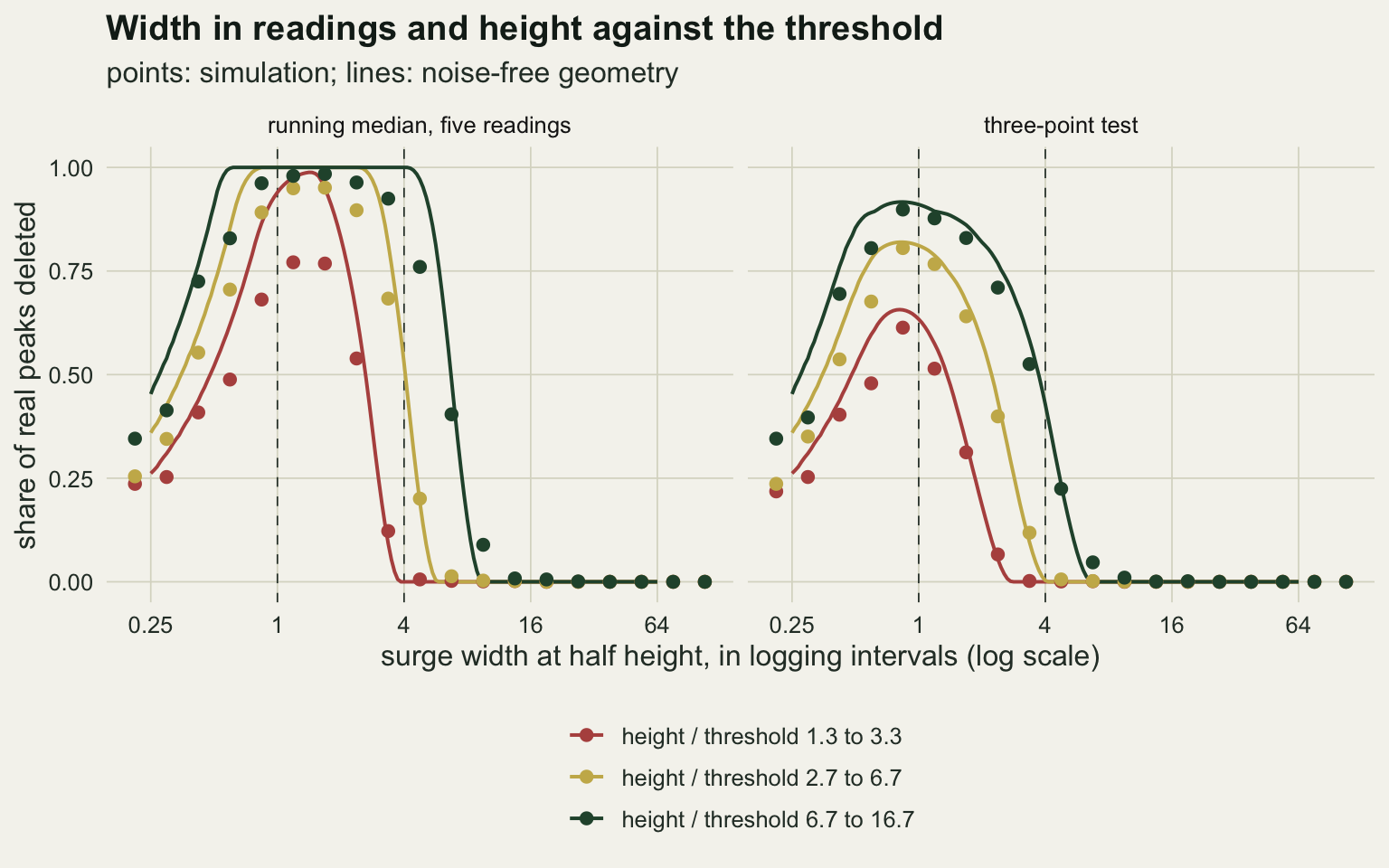
What the cleaned record says about the hot hours
qty_mean <- aggregate(. ~ iv, qty_all, mean)
qty_mean$max_raw_d <- qty_mean$max_raw - qty_mean$max_ok
qty_mean$max_qc_d  <- qty_mean$max_qc - qty_mean$max_ok
qty_mean$max_q3_d  <- qty_mean$max_q3 - qty_mean$max_ok
qty_mean$hot_raw_r <- qty_mean$hot_raw / qty_mean$hot_ok
qty_mean$hot_qc_r  <- qty_mean$hot_qc / qty_mean$hot_ok
qty_mean$hot_q3_r  <- qty_mean$hot_q3 / qty_mean$hot_ok
q_row <- function(ivv) qty_mean[qty_mean$iv == ivv, ]
q5 <- q_row(5); q60 <- q_row(60); q30 <- q_row(30)
The two rates matter because of what is reported from the cleaned record. The chunk compares each logged record with the same logged record without artefacts, so that the effect of cleaning is separated from the separate loss of peak height that a coarse interval causes by itself. For reference, that loss is present: the artefact-free record maximum averages 23.08 degrees at 5 minutes and 22.64 degrees at 60 minutes.
With no quality control the artefacts inflate both summaries. The record maximum is 1.50 degrees too high on average at 5 minutes and 0.39 too high at 60 minutes, and the hours above 20 degrees are 1.17 and 1.15 times the artefact-free value. After the fixed 1.5-degree running-median test the 5-minute record is restored: its maximum changes by 0.00 degrees and its hot hours ratio is 0.996. The 30-minute record comes out with a maximum 0.41 degrees too low and 0.79 of its hot hours. The hourly record comes out with a maximum 1.25 degrees too low and only 0.39 of its hours above 20 degrees. The three-point test does less harm and still some: the hourly record keeps 0.72 of its hot hours and its maximum is 0.58 degrees too low.
The direction of the error changes sign with cleaning, and at 60 minutes the cleaned record is further from the truth than the raw one on both summaries, after either test. That comparison depends on how frequent and how large the artefacts are relative to the surges, and a record with fewer artefacts would make the raw series look better still. What does not depend on those choices is that the real readings the test removes are the ones that stand furthest above their neighbours, which on this record means surge crests, and surge crests are where the hours above a threshold come from.
ext_df <- rbind(
  data.frame(iv = qty_mean$iv, what = "change in record maximum (degrees)",
             val = qty_mean$max_raw_d, arm = "no quality control"),
  data.frame(iv = qty_mean$iv, what = "change in record maximum (degrees)",
             val = qty_mean$max_qc_d, arm = "after the running-median test"),
  data.frame(iv = qty_mean$iv, what = "hours above 20 degrees, ratio",
             val = qty_mean$hot_raw_r, arm = "no quality control"),
  data.frame(iv = qty_mean$iv, what = "hours above 20 degrees, ratio",
             val = qty_mean$hot_qc_r, arm = "after the running-median test"),
  data.frame(iv = qty_mean$iv, what = "change in record maximum (degrees)",
             val = qty_mean$max_q3_d, arm = "after the three-point test"),
  data.frame(iv = qty_mean$iv, what = "hours above 20 degrees, ratio",
             val = qty_mean$hot_q3_r, arm = "after the three-point test"))
ext_df$arm <- factor(ext_df$arm, levels = c("no quality control",
  "after the running-median test", "after the three-point test"))
ref_df <- data.frame(what = c("change in record maximum (degrees)",
                              "hours above 20 degrees, ratio"), ref = c(0, 1))
ggplot(ext_df, aes(iv, val, colour = arm)) +
  geom_hline(data = ref_df, aes(yintercept = ref), linetype = "dashed",
             colour = te_body) +
  geom_line(linewidth = 0.9) + geom_point(size = 2.4) +
  scale_colour_manual(values = c(te_gold, te_rust, te_forest), name = NULL) +
  scale_x_continuous(breaks = iv_set) +
  facet_wrap(~what, scales = "free_y") +
  labs(x = "logging interval (minutes)", y = NULL,
       title = "Cleaning trades one error in the extremes for another") +
  theme_datasheet() +
  theme(legend.position = "bottom")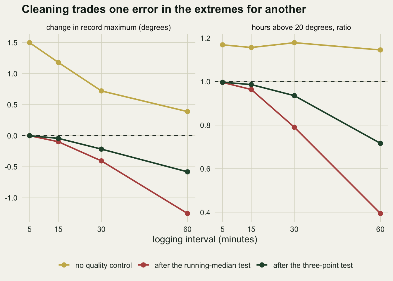
When the artefacts are much larger than any surge
big_lo <- 10
big_hi <- 15
set.seed(55123)
big_list <- lapply(seq_len(n_rep), function(r_i) {
  sr <- sim_series(90)
  lg <- log_series(sr, 12, a_lo = big_lo, a_hi = big_hi)
  data.frame(thr = thr_grid,
             c_art = vapply(thr_grid, function(h) sum(lg$dev5[lg$art] > h), 0),
             n_art = length(lg$art),
             c_pk = vapply(thr_grid, function(h) sum(lg$dev5[lg$pk] > h), 0),
             n_pk = length(lg$pk))
})
big_tab <- aggregate(cbind(c_art, n_art, c_pk, n_pk) ~ thr, do.call(rbind, big_list), sum)
big_tab$catch <- big_tab$c_art / big_tab$n_art
big_tab$del   <- big_tab$c_pk / big_tab$n_pk
big_best <- big_tab[big_tab$catch >= 0.99, ]
big_best <- big_best[which.min(big_best$del), ]
The failure above needs artefacts and surges of overlapping size. If the artefacts are a different kind of object, for instance an electrical fault that throws readings 10 to 15 degrees away, the hourly record can be cleaned by size. Rerunning the 60-minute arm with such artefacts, the threshold of 6.27 degrees catches 0.999 of 700 artefacts and deletes 0.000 of 1927 surge peaks. That test no longer uses the neighbours for anything except a baseline; it works because the largest surge, 5 degrees, is smaller than the smallest artefact. When the artefacts of a given sensor are known to be that large, the logging interval stops mattering for spikes; when they are the size of the events being studied, it decides everything.
What to report
State the logging interval next to the quality control rule, and state the threshold in physical units. A threshold written as a multiple of the median absolute deviation of the differences changes its meaning with the interval: the same k of 6 is 0.59 degrees at 5 minutes and 4.76 degrees at 60 minutes in this simulation.
Report the number of readings flagged, and keep them in the data file as a flag column rather than deleting them. The software Horsburgh and colleagues describe records each correction so that the editing steps can be traced and repeated, and a record of that kind is what allows a later reader to count how many flagged readings were surge crests.
Compare the typical width of the events of interest with the interval before the logger is deployed. If the events are less than about four readings wide at the planned interval and stand no more than about three times the threshold, a five-reading running-median test will remove some of them, and the rate climbs steeply below that; taller events relative to the threshold survive only when wider, and a three-point test tolerates events down to about three readings here. The width can be checked with the formula above before any data exist. The cheap repair is a shorter interval; a flagged reading on a coarse record should be reviewed against an independent record, such as rainfall, stage, or a second logger, before it is removed.
Report extremes and threshold exceedances with and without the flagged readings. At an hourly interval in this simulation the version of the hours above 20 degrees without the readings the running-median test flags is 0.39 of the artefact-free value, a factor of 2.5, and 0.72 after the three-point test, and a reader needs both to judge the result.
Honest limits
Only one kind of sensor failure is simulated. One-reading spikes are the failure this test is built for, but Leigh and colleagues also classify sudden shifts, drift, periods of anomalously low or high variability, impossible values and missing observations in their river records. Those need different tests, and a spike test does nothing about them; the rates above say nothing about how common spikes are relative to the rest. For a stream temperature logger the common failures are burial, drying out and drift, which span many readings; isolated one-reading glitches are more typical of turbidity or conductivity probes, so half a per cent of readings is a generous spike rate for temperature.
The surges are symmetric Gaussian bumps. Storm surges in streams often rise quickly and fall slowly, so the crest of an asymmetric surge has one neighbour much closer in value than the other. That helps a duration-aware rule on the falling side and hurts it on the rising side, and the size of the net effect was not measured.
The logger takes an instantaneous reading. Many loggers can instead store the average of fast samples over the interval. Averaging shrinks a one-reading artefact that lasted a second almost to nothing, and also flattens the surge crest, so an averaging logger changes both rates at once and needs its own simulation.
The artefacts are independent of the surges and of each other, their size range overlaps the surge heights by design, and they make up half a per cent of readings. A sensor that fails more often during storms, when debris strikes it or the water level drops, would concentrate artefacts on exactly the readings the test is most likely to misjudge.
Four of the rules use a five-reading running median and one a three-reading window. A wider window covers more time at a coarse interval and follows the diel curve less closely, and it was not run. The three-point test does less damage to crests, but by its formula two adjacent artefacts of similar size score as a plateau and neither is flagged. The fixed threshold of 1.5 degrees, the half-threshold rule for the neighbours, the diel amplitude and the noise level are single choices, and the sweeps cover threshold, surge width and surge height against the threshold, not those.
The median surge widths of 45, 90 and 180 minutes were chosen to bracket the surges Nelson and Palmer describe for urban streams. Conductivity pulses from road salt, dissolved oxygen swings in a eutrophic pond or soil temperature under a passing cloud have their own widths, and the width in readings carries over only together with the height of the event against the threshold, not the rates at any particular interval.
Surges here arrive on about a third of days, more often than the at most one summer day in ten Nelson and Palmer report for their most urbanised streams. The same records without surges have 0 hours (at every interval) above 20 degrees, so every hot hour is a surge crest, and the hot-hours ratio after cleaning mostly restates the crest deletion rate.
References
Campbell JL, Rustad LE, Porter JH, Taylor JR, Dereszynski EW, Shanley JB, Gries C, Henshaw DL, Martin ME, Sheldon WM, Boose ER 2013 BioScience 63(7):574-585 (10.1525/bio.2013.63.7.10)
Horsburgh JS, Reeder SL, Jones AS, Meline J 2015 Environmental Modelling and Software 70:32-44 (10.1016/j.envsoft.2015.04.002)
Leigh C, Alsibai O, Hyndman RJ, Kandanaarachchi S, King OC, McGree JM, Neelamraju C, Strauss J, Talagala PD, Turner RDR, Mengersen K, Peterson EE 2019 Science of the Total Environment 664:885-898 (10.1016/j.scitotenv.2019.02.085)
Nelson KC, Palmer MA 2007 Journal of the American Water Resources Association 43(2):440-452 (10.1111/j.1752-1688.2007.00034.x)
Wong A, Keeley R, Carval T, Argo Data Management Team 2025 Argo quality control manual for CTD and trajectory data, version 3.9 (Ifremer; 10.13155/33951)