Species distribution modelling with GLM in R

Fit a species distribution model in R with a binomial GLM: draw presence and background points, model humped responses, and map predicted habitat suitability.

A species distribution model (SDM) links records of where a species has been found to the environmental conditions at those places, then uses that relationship to map suitability across a landscape. The simplest useful version is a binomial GLM: contrast the conditions at occurrence points against the conditions available in the wider region, and let the fitted probabilities stand in for relative suitability. This post builds one end to end on a synthetic landscape, so every number is reproducible, and keeps the moving parts visible: the predictors, the training points, the model, and the prediction.

We work with a simulated region rather than downloaded data so the “true” niche is known and the model can be checked against it. The workflow itself is identical for real occurrence records; cleaning those records is covered separately.

library(terra)
library(sf)
library(dplyr)
library(ggplot2)
library(patchwork)

pal_paper <- "#f5f4ee"; pal_ink <- "#16241d"; pal_body <- "#2c3a31"
pal_forest <- "#275139"; pal_label <- "#46604a"; pal_line <- "#dad9ca"; pal_faint <- "#5d6b61"
theme_te <- function(base_size = 12) {
  theme_minimal(base_size = base_size) +
    theme(text = element_text(colour = pal_body),
          plot.title = element_text(colour = pal_ink, face = "bold", size = rel(1.05)),
          plot.subtitle = element_text(colour = pal_faint),
          axis.title = element_text(colour = pal_label), axis.text = element_text(colour = pal_body),
          panel.grid.minor = element_blank(),
          panel.grid.major = element_line(colour = pal_line, linewidth = 0.3),
          strip.text = element_text(colour = pal_ink, face = "bold"),
          legend.title = element_text(colour = pal_label),
          plot.background = element_rect(fill = pal_paper, colour = NA),
          panel.background = element_rect(fill = "white", colour = NA),
          legend.key = element_rect(fill = pal_paper, colour = NA))
}
as_df <- function(r, nm) { d <- as.data.frame(r, xy = TRUE); names(d)[3] <- nm; d }

A landscape and two predictors

The region is an 80 by 80 grid with two environmental layers. Temperature runs warm in the south and cool in the north; precipitation runs dry in the west and wet in the east. Each layer is a smooth trend plus spatially smoothed noise, which gives the gentle texture real climate surfaces have. The smoothing uses a moving window (focal), so neighbouring cells are correlated rather than independent.

set.seed(42)
r_template <- rast(nrows = 80, ncols = 80, xmin = 0, xmax = 80, ymin = 0, ymax = 80)
xy <- xyFromCell(r_template, 1:ncell(r_template))

# temperature: warm in the south (low y), cool in the north, plus smooth noise
temp_trend <- 22 - 0.18 * xy[, "y"]
temp_noise <- rast(r_template); values(temp_noise) <- rnorm(ncell(r_template), 0, 2)
temp_noise <- focal(temp_noise, w = 9, fun = mean, na.rm = TRUE)
temp <- rast(r_template); values(temp) <- temp_trend
temp <- temp + temp_noise; names(temp) <- "temp"

# precipitation: dry in the west, wet in the east, plus smooth noise
prec_trend <- 500 + 5 * xy[, "x"]
prec_noise <- rast(r_template); values(prec_noise) <- rnorm(ncell(r_template), 0, 60)
prec_noise <- focal(prec_noise, w = 9, fun = mean, na.rm = TRUE)
prec <- rast(r_template); values(prec) <- prec_trend
prec <- prec + prec_noise; names(prec) <- "prec"

env <- c(temp, prec)
round(range(values(temp)), 1)   # temperature span

[1]  7.0 22.5

round(range(values(prec)), 0)   # precipitation span

[1] 486 915

Temperature spans roughly 7 to 22.5 degrees and precipitation 486 to 915 mm, so both gradients cover a wide enough range for a species to have a clear preference inside them.

d_temp <- as_df(env[["temp"]], "value")
d_prec <- as_df(env[["prec"]], "value")
gg_temp <- ggplot(d_temp, aes(x, y, fill = value)) + geom_raster() +
  scale_fill_gradient(low = "#c9b458", high = "#1d5b4e", name = "C") +
  coord_equal(expand = FALSE) + labs(title = "Temperature", x = "Easting", y = "Northing") +
  theme_te(11)
gg_prec <- ggplot(d_prec, aes(x, y, fill = value)) + geom_raster() +
  scale_fill_gradient(low = "#c9b458", high = "#1d5b4e", name = "mm") +
  coord_equal(expand = FALSE) + labs(title = "Precipitation", x = "Easting", y = NULL) +
  theme_te(11)
(gg_temp | gg_prec) +
  plot_annotation(title = "Environmental predictors across the study region",
                  theme = theme(plot.title = element_text(colour = pal_ink, face = "bold", size = 14),
                                plot.background = element_rect(fill = pal_paper, colour = NA)))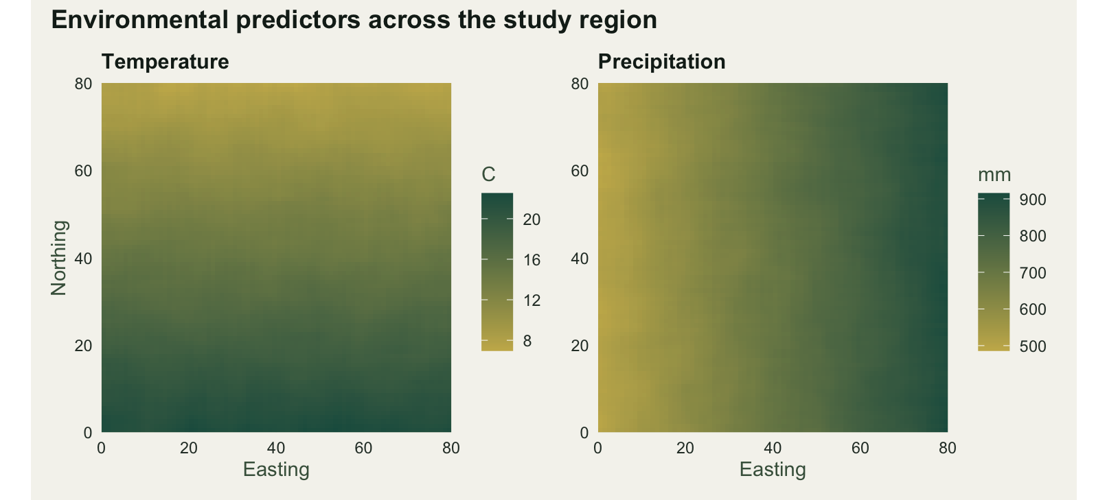

Figure 1: The two environmental predictors. Each panel has its own colour scale.

The species and its records

The species prefers moderate temperature (optimum near 15 degrees) and fairly wet conditions (optimum near 800 mm), with a Gaussian falloff away from each optimum. Multiplying the two Gaussian responses gives a true suitability surface. In a real study this surface is unknown; here it is the yardstick.

Occurrence records are then drawn as 300 locations sampled in proportion to that suitability. This mimics how presence data accumulate: more records where conditions are good, fewer where they are poor, and none of the true absences that a designed survey would give.

temp_opt <- 15; temp_tol <- 2.2
prec_opt <- 800; prec_tol <- 110
suit_true <- exp(-((values(temp) - temp_opt)^2) / (2 * temp_tol^2)) *
             exp(-((values(prec) - prec_opt)^2) / (2 * prec_tol^2))

set.seed(101)
pres_cells <- sample(ncell(r_template), 300, prob = suit_true, replace = FALSE)
pres_xy <- xy[pres_cells, ]

A binomial GLM needs something to contrast the presences against. With presence-only data that role is played by background points: a random sample of the conditions available across the region, labelled zero. They are not asserted absences; they describe what the landscape offers, so the model can ask whether presences fall in unusually suitable parts of it.

set.seed(202)
bg_cells <- sample(ncell(r_template), 1000)

pres_df <- data.frame(pa = 1, temp = values(temp)[pres_cells], prec = values(prec)[pres_cells])
bg_df   <- data.frame(pa = 0, temp = values(temp)[bg_cells],  prec = values(prec)[bg_cells])
dat <- rbind(pres_df, bg_df)
dat <- dat[complete.cases(dat), ]
c(rows = nrow(dat), presences = sum(dat$pa), background = sum(dat$pa == 0))

      rows  presences background 
      1300        300       1000 

Fitting the model

The model is a binomial GLM with a second-order polynomial in each predictor. The quadratic terms matter: a species with an optimum has a humped response, and a purely linear term can only make suitability rise or fall monotonically. poly(temp, 2) supplies the linear and squared terms in an orthogonal basis, which keeps the two columns uncorrelated and the fit numerically stable.

m <- glm(pa ~ poly(temp, 2) + poly(prec, 2), data = dat, family = binomial)
round(coef(m), 3)

   (Intercept) poly(temp, 2)1 poly(temp, 2)2 poly(prec, 2)1 poly(prec, 2)2 
        -1.912         -3.734        -52.384         31.020        -15.176 

The negative second-order coefficients on both predictors are the signature of a humped response: suitability peaks somewhere in the middle of each gradient and drops on either side. A quick fit summary confirms the model has captured real structure rather than noise.

dev_expl <- 1 - m$deviance / m$null.deviance
round(100 * dev_expl, 1)   # deviance explained, per cent

[1] 22

The model explains about 22 per cent of the deviance. That figure looks modest, but with a large random background the null model is already spread thinly across the whole region, so a fifth of the deviance is a substantial signal for presence-background data. Deviance explained is a within-sample descriptor, not a validation; honest performance needs held-out data, which the evaluation post takes up.

Predicting and mapping suitability

terra::predict runs the fitted model over every raster cell, applying the stored polynomial basis to the temperature and precipitation there. With type = "response" the output is on the probability scale, giving a continuous suitability surface.

pred_r <- terra::predict(env, m, type = "response", na.rm = TRUE)
round(range(values(pred_r), na.rm = TRUE), 3)      # suitability range

[1] 0.000 0.574

round(cor(values(pred_r)[, 1], suit_true), 3)      # agreement with the true surface

      temp
[1,] 0.969

Predicted suitability ranges from near zero to about 0.57, and it correlates with the hidden true surface at 0.969. The model has recovered the niche well, which is the payoff of a controlled simulation: on real data that check is impossible, and the map is all you get.

d_pred <- as_df(pred_r, "suit")
d_pres <- as.data.frame(pres_xy); names(d_pres) <- c("x", "y")
ggplot(d_pred, aes(x, y)) +
  geom_raster(aes(fill = suit)) +
  geom_point(data = d_pres, colour = "#b5534e", size = 0.7, alpha = 0.8) +
  scale_fill_gradient(low = pal_paper, high = pal_forest, name = "Suitability", limits = c(0, NA)) +
  coord_equal(expand = FALSE) +
  labs(title = "Predicted habitat suitability with occurrence records",
       x = "Easting", y = "Northing") +
  theme_te(12)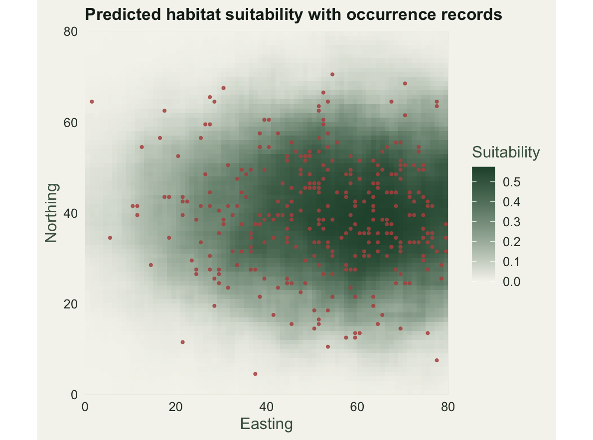

Figure 2: Predicted habitat suitability with the 300 occurrence records overlaid.

Reading the response curves

Coefficients on an orthogonal polynomial are hard to interpret directly. The clearer view is a partial response curve: vary one predictor across its range, hold the other at its median, and predict. This is the shape the model believes the species follows along each axis.

temp_seq <- seq(min(dat$temp), max(dat$temp), length.out = 100)
pr_t <- predict(m, data.frame(temp = temp_seq, prec = median(dat$prec)), type = "response")
prec_seq <- seq(min(dat$prec), max(dat$prec), length.out = 100)
pr_p <- predict(m, data.frame(temp = median(dat$temp), prec = prec_seq), type = "response")
c(temp_peak = round(temp_seq[which.max(pr_t)], 1),
  prec_peak = round(prec_seq[which.max(pr_p)], 0))

temp_peak prec_peak 
     14.8     811.0 

d_resp <- rbind(data.frame(x = temp_seq, y = pr_t, predictor = "Temperature (C)"),
                data.frame(x = prec_seq, y = pr_p, predictor = "Precipitation (mm)"))
ggplot(d_resp, aes(x, y)) +
  geom_line(colour = pal_forest, linewidth = 1) +
  facet_wrap(~predictor, scales = "free_x") +
  labs(title = "Partial response curves from the fitted GLM",
       subtitle = "Other predictor held at its median",
       x = NULL, y = "Predicted suitability") +
  theme_te(12)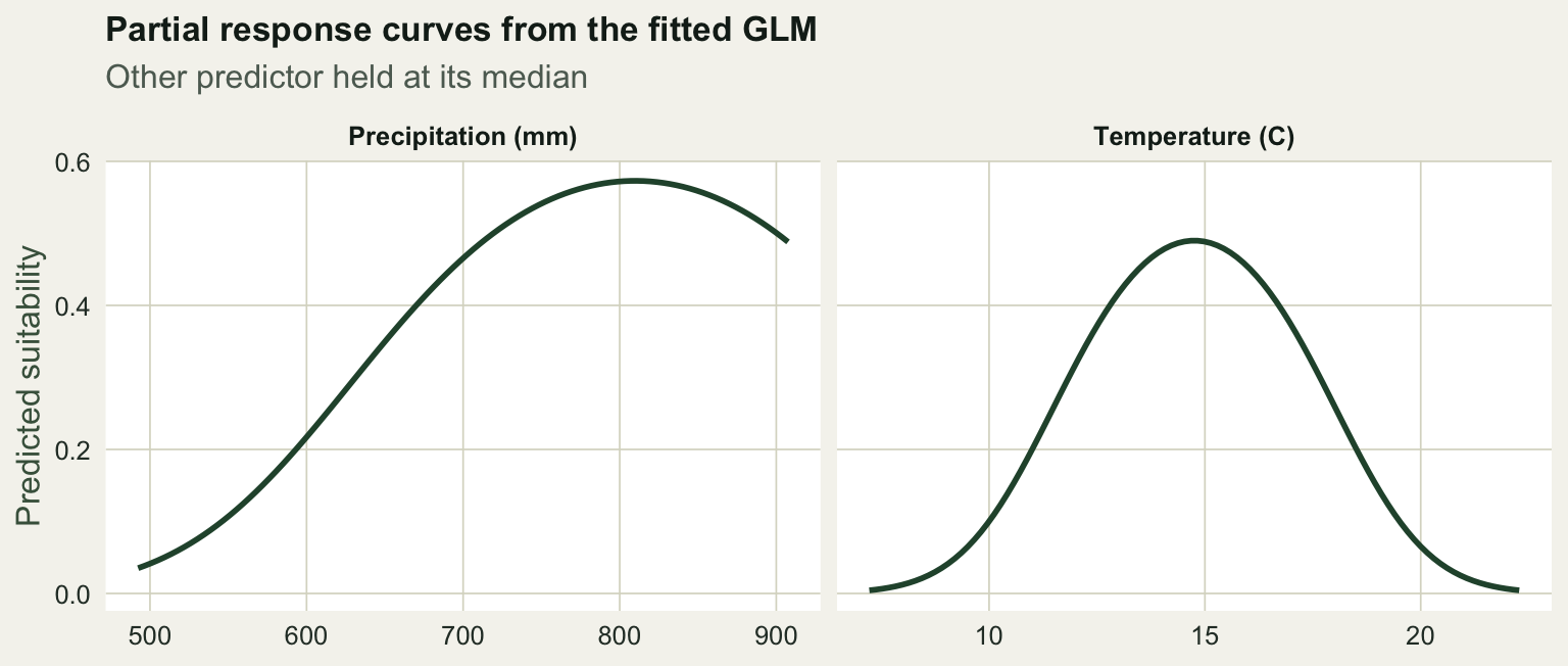

Figure 3: Partial response curves. The peak of each curve estimates the species optimum on that axis.

The temperature curve peaks at 14.8 degrees and the precipitation curve at 811 mm, within a whisker of the true optima of 15 and 800. The quadratic GLM has reconstructed both preferences from nothing but occurrence and background points, which is the whole idea of a correlative SDM.

What this leaves out

A working model is not a trustworthy one. Three gaps are worth naming, each handled in its own tutorial. First, the background is a modelling choice: how many points, and drawn from where, changes the fit. Second, the deviance figure here is in-sample; real performance needs held-out data and metrics such as AUC and TSS. Third, occurrence records are spatially clustered, so a naive random split flatters a model by testing it on points next to its training data. The synthetic landscape also hides the everyday problems of real predictors, collinearity among climate layers and extrapolation beyond the sampled range, that decide whether an SDM generalises.

Treat this post as the skeleton: presence versus background, a flexible response, a prediction on the response scale. The posts that follow put the flesh on it.

References

• Guisan A, Zimmermann NE 2000. Ecological Modelling 135(2-3):147-186 (10.1016/S0304-3800(00)00354-9)
• Elith J, Leathwick JR 2009. Annual Review of Ecology, Evolution, and Systematics 40:677-697 (10.1146/annurev.ecolsys.110308.120159)
• Guisan A, Thuiller W, Zimmermann NE 2017. Habitat Suitability and Distribution Models with Applications in R. Cambridge University Press (ISBN 978-0-521-75836-9)
• Pebesma E 2018. The R Journal 10(1):439-446 (10.32614/RJ-2018-009)

Related tutorials

• Cleaning GBIF and iNaturalist records in R
• Logistic regression for presence-absence data
• GAM species response curves with mgcv
• Imperfect detection and occupancy bias in R