library(ggplot2)

te_paper  <- "#f5f4ee"
te_ink    <- "#16241d"
te_body   <- "#2c3a31"
te_forest <- "#275139"
te_rust   <- "#b5534e"
te_gold   <- "#c9b458"
te_line   <- "#dad9ca"

theme_datasheet <- function() {
  theme_minimal(base_size = 12) +
    theme(plot.background  = element_rect(fill = te_paper, colour = NA),
          panel.background = element_rect(fill = te_paper, colour = NA),
          panel.grid.major = element_line(colour = te_line, linewidth = 0.3),
          panel.grid.minor = element_blank(),
          text             = element_text(colour = te_body),
          plot.title       = element_text(colour = te_ink, face = "bold"),
          plot.subtitle    = element_text(colour = te_body),
          axis.text        = element_text(colour = te_body))
}Separable space-time covariance, tested
R
spatial
time series
covariance
simulation
ecology tutorial
A separable space-time covariance turns one Cholesky into a Kronecker product, but fixes one spatial range for every time lag. Measuring the cost in R.
Fifty soil moisture loggers are scattered over a twenty kilometre square of upland grazing, and each has returned forty monthly means. The analysis everyone reaches for treats the two thousand values as one multivariate normal vector with a covariance that depends on the distance between two loggers and on the number of months between two readings. The next step is almost always the same too: write that covariance as a spatial correlation times a temporal correlation, because the two thousand by two thousand matrix then never has to be factorised, and the likelihood runs in a blink.
That product is called a separable covariance, and the saving is real. What gets less attention is what the product says about the landscape. If \(C(h, u) = C_s(h)\,C_t(u)\), then the correlation between two loggers a distance \(h\) apart, read at a lag of \(u\) months, is the same function of \(h\) at every \(u\). The spatial range of the moisture anomaly is fixed; a wet patch one month does not spread into a wider wet patch three months later. That is an ecological statement, and it is testable.
The site has already met both halves separately. Generalised least squares for spatial data fits a purely spatial exponential correlation to one snapshot of plots with nlme, and repeated measures and temporal correlation puts an AR(1) structure on the residuals within each plot and treats plots as independent. Neither multiplies space and time together. The variogram and the GP kernel shows that a spatial covariance function and a Gaussian process kernel are one object; the covariance functions here are that object with a time axis added. The Kronecker product itself is not new on the site either: fitting a MAR(1) model uses it to solve the Lyapunov equation for the stationary covariance of a community, and behavioural syndromes in R builds a trait by occasion covariance as a sum of two Kronecker products. Both of those use the product as algebra for one matrix equation. Here it is a modelling assumption about how correlation in space and correlation in time interact, and the question is what that assumption costs when it is wrong.
The post checks the Kronecker identity numerically, measures the speed-up, fits a separable model by maximum likelihood to data generated from a non-separable covariance of the kind Gneiting introduced in 2002, and then tries the obvious diagnostic, the ratio \(C(h,u)\,C(0,0) / \{C(h,0)\,C(0,u)\}\), which equals one at every \(h\) and \(u\) under separability.
Two covariance functions with the same margins
The non-separable truth is a member of the Gneiting class with an exponential decay in space and a Cauchy-type decay in time,
\[C(h, u) = \frac{\sigma^2}{a|u| + 1}\,\exp\left(-\frac{c\,h}{(a|u| + 1)^{\beta/2}}\right),\]
which is a valid covariance in two spatial dimensions for any \(\beta\) between zero and one. The parameter \(\beta\) is the interaction. At \(\beta = 0\) the denominator inside the exponential disappears and the function factorises into \(\sigma^2 \exp(-c h)\) times \(1/(a|u|+1)\): a separable covariance. At \(\beta = 1\) the spatial decay rate at lag \(u\) is divided by the square root of \(a|u|+1\), so the spatial range grows with the time lag. The two versions share both margins exactly, \(C(h, 0)\) and \(C(0, u)\), and differ only in how space and time combine. That makes the comparison clean: a separable model with the right families for both margins is misspecified in the interaction and in nothing else.
n_site <- 50                        # loggers
n_time <- 40                        # monthly means
side_km <- 20                       # side of the square
c_sp   <- 1 / 3                     # spatial decay rate per km at lag zero
a_tm   <- 0.5                       # temporal scale per month
beta_ns <- 1                        # interaction of the non-separable truth
sig2   <- 1                         # variance
n_obs  <- n_site * n_time

set.seed(3071)
site_xy <- cbind(runif(n_site, 0, side_km), runif(n_site, 0, side_km))
dist_km <- as.matrix(dist(site_xy))
lag_mo  <- abs(outer(seq_len(n_time), seq_len(n_time), "-"))

gneiting_cov <- function(h, u, beta) {
  psi <- a_tm * u + 1
  sig2 * exp(-c_sp * h / psi^(beta / 2)) / psi
}

dist_med  <- median(dist_km[upper.tri(dist_km)])
cor_lag1  <- gneiting_cov(0, 1, beta_ns) / sig2
cor_lag3  <- gneiting_cov(0, 3, beta_ns) / sig2
prac_fac  <- -log(0.05)
range_at  <- function(u, beta) prac_fac * (a_tm * u + 1)^(beta / 2) / c_sp
range_0   <- range_at(0, beta_ns)
range_3   <- range_at(3, beta_ns)
range_6   <- range_at(6, beta_ns)
The design constants were fixed before anything was simulated. The loggers sit at random in the square, with a median separation of 9.4 km. The temporal correlation at one month is 0.667 and at three months 0.400. The spatial correlation falls to five per cent at 9.0 km for two readings taken in the same month; under the non-separable truth that practical range is 14.2 km at a lag of three months and 18.0 km at six. Under the separable version it is 9.0 km at every lag.
The Kronecker product is exact, and the saving is large
Stack the data month by month, so that the first 50 values are the loggers in month one. The covariance of that vector under a separable model is the Kronecker product \(\Sigma_t \otimes \Sigma_s\) of a 40 by 40 temporal matrix and a 50 by 50 spatial one. Van Loan’s 2000 review collects the identities that make this useful: the Cholesky factor of a Kronecker product is the Kronecker product of the factors, the inverse is the product of the inverses, and the log determinant is \(n_s \log|\Sigma_t| + n_t \log|\Sigma_s|\). The quadratic form in the likelihood then needs only two triangular solves on a 50 by 40 data matrix.
sp_cor <- exp(-c_sp * dist_km)
tm_cor <- 1 / (a_tm * lag_mo + 1)
big_cov <- kronecker(tm_cor, sp_cor)

chol_full <- chol(big_cov)
chol_kron <- kronecker(chol(tm_cor), chol(sp_cor))
chol_gap  <- max(abs(chol_full - chol_kron))

set.seed(3072)
y_test <- as.vector(crossprod(chol_kron, rnorm(n_obs)))

nll_full <- function(y, r_up) {
  z_vec <- backsolve(r_up, y, transpose = TRUE)
  sum(log(diag(r_up))) + 0.5 * sum(z_vec^2)
}
nll_kron <- function(y_mat, rs_up, rt_up) {
  w_mat <- backsolve(rs_up, y_mat, transpose = TRUE)
  w_mat <- t(backsolve(rt_up, t(w_mat), transpose = TRUE))
  ncol(y_mat) * sum(log(diag(rs_up))) + nrow(y_mat) * sum(log(diag(rt_up))) +
    0.5 * sum(w_mat^2)
}
ll_gap <- abs(nll_full(y_test, chol_full) -
              nll_kron(matrix(y_test, n_site, n_time), chol(sp_cor), chol(tm_cor)))
ll_val <- nll_full(y_test, chol_full)
The two Cholesky factors of the 2000 by 2000 matrix, one computed directly and one assembled from the two small factors, differ by at most 2.16e-15 in any entry. The negative log-likelihood of a simulated data set is -146.9189 computed either way, with an absolute difference of 1.14e-13. Both gaps are rounding.
n_time_grid <- c(5, 10, 20, 30, 40)
n_full_rep  <- c(200, 20, 2, 1, 1)    # repeats so that no timing is near the clock resolution
n_small_rep <- 500

time_tab <- do.call(rbind, lapply(seq_along(n_time_grid), function(j) {
  k_t   <- n_time_grid[j]
  tm_k  <- 1 / (a_tm * abs(outer(seq_len(k_t), seq_len(k_t), "-")) + 1)
  big_k <- kronecker(tm_k, sp_cor)
  t_full <- system.time(for (i in seq_len(n_full_rep[j])) chol(big_k))[["elapsed"]] /
    n_full_rep[j]
  t_kron <- system.time(for (i in seq_len(n_small_rep)) {
    chol(sp_cor); chol(tm_k)
  })[["elapsed"]] / n_small_rep
  data.frame(n_time = k_t, n_obs = k_t * n_site, full = t_full, kron = t_kron)
}))

# leading-order floating point operation counts (deterministic)
flop_chol  <- n_obs^3 / (n_site^3 + n_time^3)
flop_full  <- n_obs^3 / 3 + n_obs^2 / 2
flop_kron  <- (n_site^3 + n_time^3) / 3 + (n_time * n_site^2 + n_site * n_time^2) / 2
flop_lik   <- flop_full / flop_kron
share_sp40 <- n_site^3 / (n_site^3 + n_time^3)
rise_flop  <- (n_site^3 + n_time^3) / (n_site^3 + min(n_time_grid)^3)

# one full likelihood evaluation each way, building the correlation matrices included
n_lik_full <- 2
n_lik_kron <- 500
y_mat_test <- matrix(y_test, n_site, n_time)
t_lik_full <- system.time(for (i in seq_len(n_lik_full)) {
  nll_full(y_test, chol(kronecker(1 / (a_tm * lag_mo + 1), exp(-c_sp * dist_km))))
})[["elapsed"]] / n_lik_full
t_lik_kron <- system.time(for (i in seq_len(n_lik_kron)) {
  nll_kron(y_mat_test, chol(exp(-c_sp * dist_km)), chol(1 / (a_tm * lag_mo + 1)))
})[["elapsed"]] / n_lik_kron
speed_lik   <- t_lik_full / t_lik_kron
speed_order <- 10^round(log10(speed_lik))
var_gmean   <- sum(big_cov) / n_obs^2
rm(big_cov, chol_full)
The size of the saving is best stated as a count of floating point operations, because that number does not depend on the computer. A Cholesky decomposition costs a third of the cube of the dimension, so the full decomposition needs 42328 times as many operations as the two small ones together. One evaluation of the likelihood also needs the triangular solves, which are cheap for the full matrix but make up most of the work in the Kronecker route; counted to leading order, a whole evaluation is 17442 times cheaper through the factors.
Timing the same two likelihood evaluations on the machine that knitted this page, with the correlation matrices built inside each call, gave a ratio of the order of 10000. Treat that only as an order of magnitude. The measured ratio changes between runs of the same code, and much more between computers: an optimised, multithreaded linear algebra library speeds up a two thousand by two thousand decomposition many times over and a fifty by fifty one hardly at all, and the fixed cost of each call into R weighs heavily on the small problem. The figure below times the decompositions alone as the number of months grows. The Kronecker line changes little, and the operation count says why: the fifty by fifty spatial factor does not grow with the number of months and is 66 per cent of the decomposition work even at forty months, so going from 5 to 40 months should raise that cost by only a factor of 1.51, before the fixed overhead of the calls is added.
time_long <- rbind(
  data.frame(n_time = time_tab$n_time, sec = time_tab$full,
             route = "full matrix"),
  data.frame(n_time = time_tab$n_time, sec = time_tab$kron,
             route = "two Kronecker factors"))

ggplot(time_long, aes(n_time, sec, colour = route)) +
  geom_line(linewidth = 0.9) +
  geom_point(size = 2.4) +
  scale_y_log10(breaks = 10^(-4:0),
                labels = c("0.0001", "0.001", "0.01", "0.1", "1")) +
  scale_colour_manual(values = c(te_rust, te_forest), name = NULL) +
  labs(x = "months (fifty sites in every case)",
       y = "seconds per decomposition (log scale)",
       title = "One cubic cost, two small ones",
       subtitle = "machine dependent: seconds and ratio both change with the linear algebra library") +
  theme_datasheet() +
  theme(legend.position = "bottom")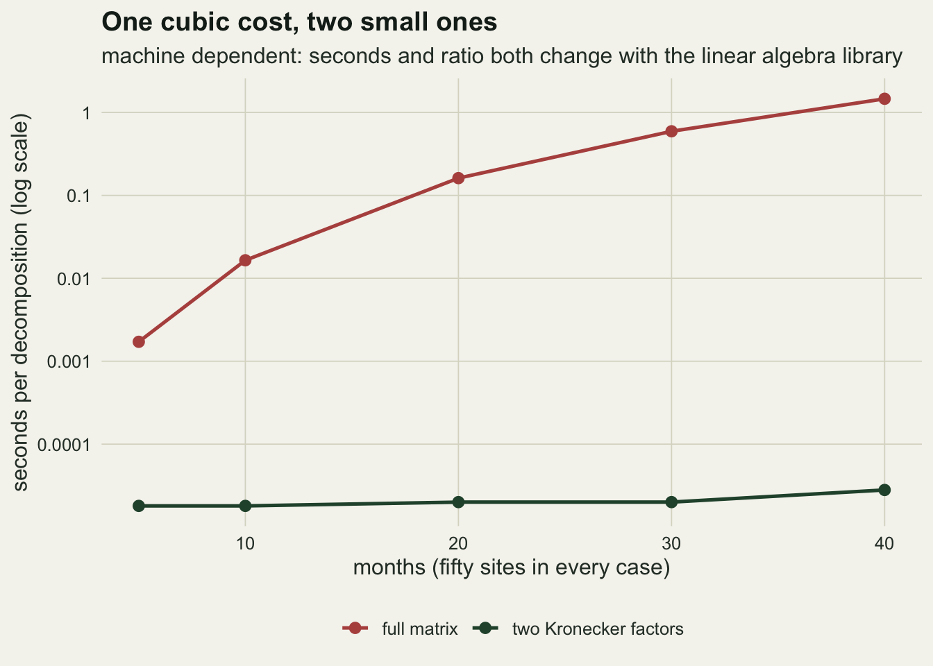
Fitting a separable model to a non-separable truth
The data sets below come from two truths with identical margins: the separable one, simulated directly through the Kronecker factor, and the non-separable one with \(\beta = 1\), for which the full matrix has to be factorised once. Each data set is fitted by maximum likelihood with the separable model and the correct marginal families. The constant mean is estimated by generalised least squares and the variance is profiled out analytically, both through the Kronecker structure, so optim works over two numbers: the spatial decay rate and the temporal scale.
n_rep <- 300

lag_block  <- kronecker(lag_mo, matrix(1, n_site, n_site))
dist_block <- kronecker(matrix(1, n_time, n_time), dist_km)
chol_ns <- chol(gneiting_cov(dist_block, lag_block, beta_ns))
rm(lag_block, dist_block)

low_sp <- t(chol(sig2 * sp_cor))
low_tm <- t(chol(tm_cor))

set.seed(3073)
sims_ns <- crossprod(chol_ns, matrix(rnorm(n_obs * n_rep), ncol = n_rep))
sims_sp <- vapply(seq_len(n_rep), function(r) {
  as.vector(low_sp %*% matrix(rnorm(n_obs), n_site) %*% t(low_tm))
}, numeric(n_obs))
rm(chol_ns)
fit_separable <- function(y_mat) {
prof_nll <- function(log_par, report = FALSE) {
rs_up <- chol(exp(-exp(log_par[1]) * dist_km))
rt_up <- chol(1 / (exp(log_par[2]) * lag_mo + 1))
one_s <- backsolve(rs_up, rep(1, n_site), transpose = TRUE)
one_t <- backsolve(rt_up, rep(1, n_time), transpose = TRUE)
w_mat <- t(backsolve(rt_up, t(backsolve(rs_up, y_mat, transpose = TRUE)),
transpose = TRUE))
one_mat <- outer(one_s, one_t)
mu_hat <- sum(w_mat * one_mat) / sum(one_mat^2)
quad <- sum((w_mat - mu_hat * one_mat)^2)
if (report) return(c(c_hat = exp(log_par[1]), a_hat = exp(log_par[2]),
s2_hat = quad / n_obs, mu_hat = mu_hat))
n_time * sum(log(diag(rs_up))) + n_site * sum(log(diag(rt_up))) +
0.5 * n_obs * log(quad / n_obs)
}
opt <- optim(log(c(c_sp, a_tm)), prof_nll, method = "L-BFGS-B",
lower = log(c(0.03, 0.01)), upper = log(c(5, 20)))
c(prof_nll(opt$par, report = TRUE), conv = opt$convergence)
}
fits_ns <- t(apply(sims_ns, 2, function(v) fit_separable(matrix(v, n_site, n_time))))
fits_sp <- t(apply(sims_sp, 2, function(v) fit_separable(matrix(v, n_site, n_time))))
n_conv_bad <- sum(fits_ns[, "conv"] != 0) + sum(fits_sp[, "conv"] != 0)
n_bound <- sum(fits_ns[, "c_hat"] < 0.031 | fits_ns[, "c_hat"] > 4.9 |
fits_ns[, "a_hat"] < 0.0101 | fits_ns[, "a_hat"] > 19.9) +
sum(fits_sp[, "c_hat"] < 0.031 | fits_sp[, "c_hat"] > 4.9 |
fits_sp[, "a_hat"] < 0.0101 | fits_sp[, "a_hat"] > 19.9)
mean_sp <- colMeans(fits_sp)
mean_ns <- colMeans(fits_ns)
se_ns <- apply(fits_ns, 2, sd) / sqrt(n_rep)
range_fit <- prac_fac / mean_ns[["c_hat"]]Every one of the 600 fits reported convergence (1 failures) and 0 estimates sat on a bound of the search box. When the truth is separable the fit does what it should: across 300 data sets the mean spatial decay rate is 0.334 against 0.333, the mean temporal scale 0.503 against 0.500, and the mean variance 1.000 against 1.
When the truth is non-separable, the same fit settles somewhere else. The mean spatial decay rate is 0.444 (Monte Carlo standard error 0.002), the temporal scale 0.658 (0.003), and the variance 0.878 (0.003). The direction is the opposite of the intuitive compromise. A reader might expect the fitted spatial range to land between the short range at lag zero and the longer ranges at later lags. It lands below all of them: the fitted practical range is 6.7 km, shorter than the 9.0 km of the truth at lag zero, and the fitted temporal correlation decays faster than the true margin too. One reading, which this post does not test, is that the likelihood of two thousand correlated values rewards predicting each value from its near neighbours in space and time, and a separable model that cannot widen its range with lag gets that local fit by making everything decay faster.
h_seq <- seq(0, 16, by = 0.1)
lag_show <- c(0, 3, 6)
truth_df <- do.call(rbind, lapply(lag_show, function(u) {
  data.frame(h = h_seq,
             cor_sp = gneiting_cov(h_seq, u, beta_ns) / gneiting_cov(0, u, beta_ns),
             curve = sprintf("truth, lag %d months", u))
}))
fit_df <- data.frame(h = h_seq, cor_sp = exp(-mean_ns[["c_hat"]] * h_seq),
                     curve = "separable fit, every lag")
curve_df <- rbind(truth_df, fit_df)
curve_df$curve <- factor(curve_df$curve, levels = c(sprintf("truth, lag %d months", lag_show),
                                                    "separable fit, every lag"))

ggplot(curve_df, aes(h, cor_sp, colour = curve, linetype = curve)) +
  geom_hline(yintercept = 0.05, colour = te_body, linewidth = 0.4, linetype = "dotted") +
  geom_line(linewidth = 1) +
  scale_colour_manual(values = c(te_forest, te_gold, te_rust, te_ink), name = NULL) +
  scale_linetype_manual(values = c("solid", "solid", "solid", "dashed"), name = NULL) +
  guides(colour = guide_legend(nrow = 2), linetype = guide_legend(nrow = 2)) +
  labs(x = "distance between loggers (km)",
       y = "spatial correlation at that lag",
       title = "The truth widens with lag; the fit cannot",
       subtitle = "dotted line: five per cent, where the practical range is read") +
  theme_datasheet() +
  theme(legend.position = "bottom")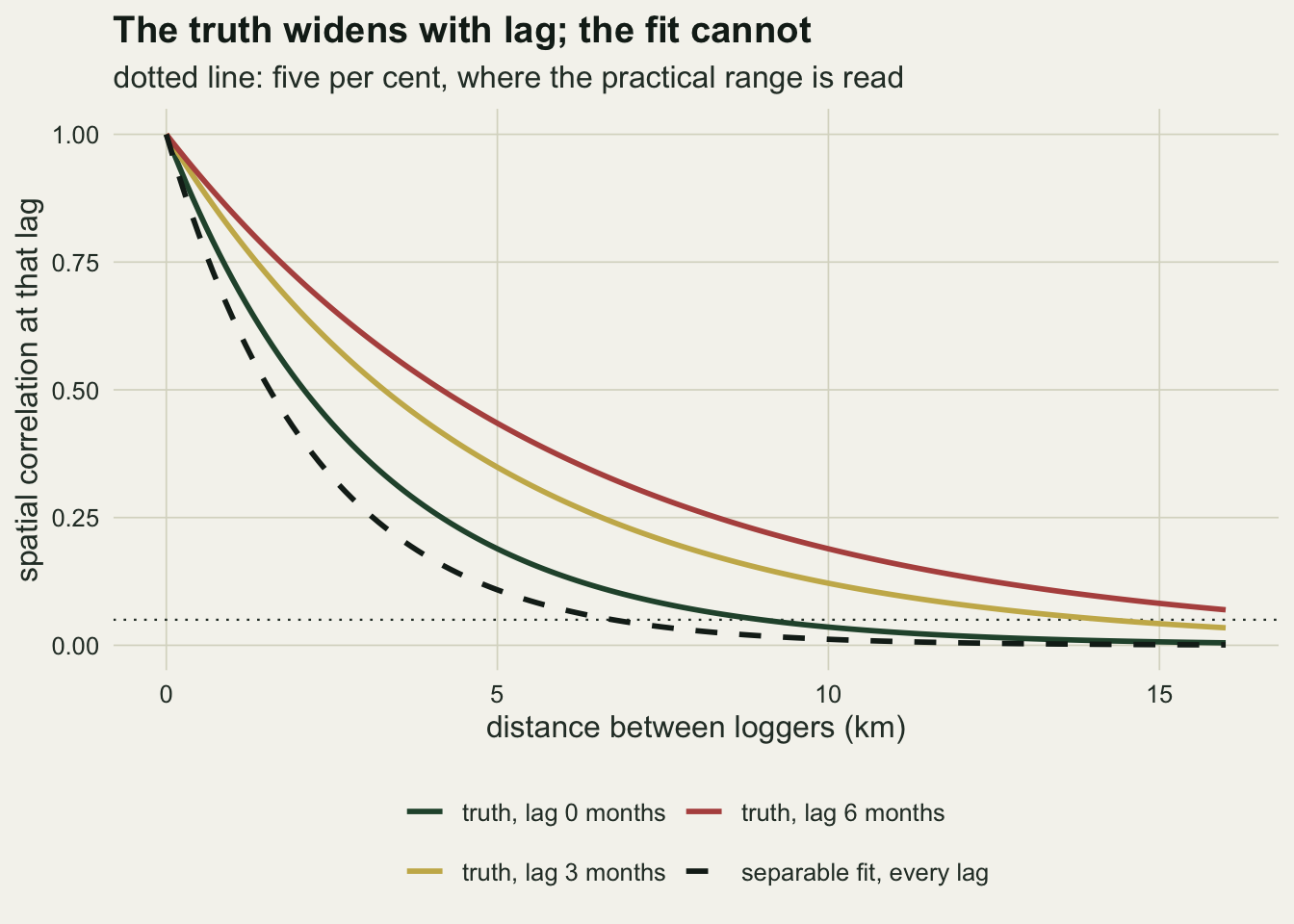
What the separable fit says about lag three
The quantity that matters for a forecast or an interpolation across months is the cross-covariance: how much a reading at one logger says about another logger some months later. The chunk below compares the covariance implied by each separable fit with the true non-separable covariance, as a ratio, across distances and at three lags.
h_grid <- seq(0, 12, by = 0.5)
lag_grid <- c(0, 1, 3)
cross_df <- do.call(rbind, lapply(lag_grid, function(u) {
  true_cov <- gneiting_cov(h_grid, u, beta_ns)
  fit_cov  <- vapply(seq_len(n_rep), function(r) {
    fits_ns[r, "s2_hat"] * exp(-fits_ns[r, "c_hat"] * h_grid) /
      (fits_ns[r, "a_hat"] * u + 1)
  }, numeric(length(h_grid)))
  ratio_mat <- fit_cov / true_cov
  data.frame(h = h_grid, lag = u, ratio = rowMeans(ratio_mat),
             lo = apply(ratio_mat, 1, quantile, 0.1),
             hi = apply(ratio_mat, 1, quantile, 0.9))
}))
pick <- function(u, h) cross_df$ratio[cross_df$lag == u & cross_df$h == h]
r3_0  <- pick(3, 0)
r3_2  <- pick(3, 2)
r3_4  <- pick(3, 4)
r3_8  <- pick(3, 8)
r0_0  <- pick(0, 0)
r0_4  <- pick(0, 4)
max_ratio_any <- max(cross_df$hi)
mono_down <- all(tapply(cross_df$ratio, cross_df$lag, function(v) all(diff(v) < 0)))
stopifnot(mono_down, max_ratio_any < 1)
true3_4 <- gneiting_cov(4, 3, beta_ns)
true_cor3_4 <- true3_4 / sig2
fit_cor3_4  <- exp(-mean_ns[["c_hat"]] * 4) / (mean_ns[["a_hat"]] * 3 + 1)
At a lag of three months the separable fit gets the covariance wrong by an amount that grows with distance, and it is wrong in one direction. For the same logger three months apart the fitted covariance is on average 0.743 of the true value; at 2 km it is 0.467, at 4 km 0.295, and at 8 km 0.118. The true covariance at 4 km and three months is 0.172, so this is not a comparison of two negligible numbers. Even at lag zero, where the separable model has the correct family, the fitted covariance is 0.878 of the truth at zero distance and 0.568 at 4 km: the right family with the wrong shape, which fits the untested reading given above.
The hypothesis this post started from was that a separable fit would overstate the lag-three cross-covariance, by something like forty per cent, since it cannot let the spatial correlation fade more slowly at longer lags and would be expected to overshoot somewhere. The measurement says the opposite: it understates it, at every distance on the grid and at every lag shown. The largest ninetieth percentile of the ratio anywhere in the figure below is 0.940, and the mean ratio falls steadily with distance at all three lags. At the mean fitted parameters, the correlation between two loggers 4 km and three months apart is 0.057, against 0.172 in the truth, so an interpolation or a forecast built on the separable fit is likely to borrow too little strength from neighbouring loggers in earlier months; no prediction was run here to measure how much.
lag_names <- c("0" = "lag 0 months", "1" = "lag 1 month", "3" = "lag 3 months")
cross_df$lag_lab <- factor(lag_names[as.character(cross_df$lag)], levels = lag_names)
ggplot(cross_df, aes(h, ratio, colour = lag_lab, fill = lag_lab)) +
  geom_hline(yintercept = 1, linetype = "dashed", colour = te_body, linewidth = 0.6) +
  geom_ribbon(aes(ymin = lo, ymax = hi), alpha = 0.18, colour = NA) +
  geom_line(linewidth = 1) +
  scale_colour_manual(values = c(te_forest, te_gold, te_rust), name = NULL) +
  scale_fill_manual(values = c(te_forest, te_gold, te_rust), name = NULL) +
  labs(x = "distance between loggers (km)",
       y = "fitted covariance / true covariance",
       title = "The separable fit understates cross-covariance",
       subtitle = "dashed line: a correct covariance") +
  theme_datasheet() +
  theme(legend.position = "bottom")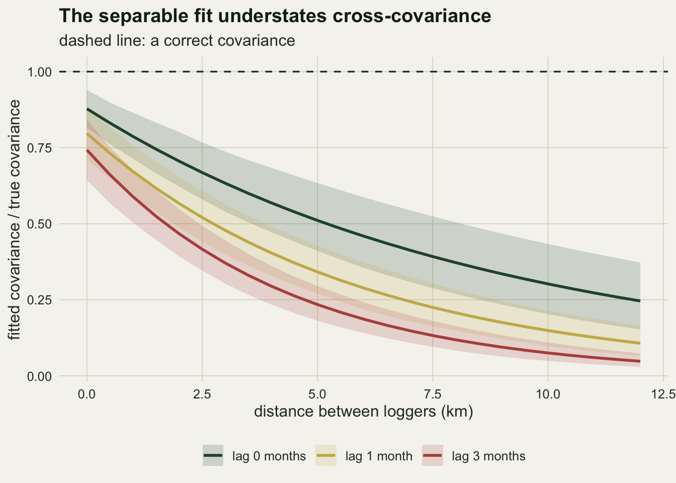
The separability ratio needs calibrating
Under separability \(C(h,u)\,C(0,0) = C(h,0)\,C(0,u)\) for every pair, so the ratio of the two sides is one. The empirical version is cheap: centre the data on its grand mean, estimate the four covariances from the logger pairs and the month pairs, and divide. The distance band and lag were fixed from the design before any data were simulated: logger pairs from 2 to 6 km apart, where the true covariance is still well away from zero, at a lag of three months. Under the non-separable truth the population ratio, averaged over the pairs in that band, is the number printed below.
band_lo <- 2
band_hi <- 6
lag_use <- 3
in_band <- dist_km >= band_lo & dist_km < band_hi
n_pairs <- sum(in_band[upper.tri(in_band)])

emp_ratio <- function(y_mat, centre = TRUE) {
  if (centre) y_mat <- y_mat - mean(y_mat)
  cov_0 <- tcrossprod(y_mat) / n_time
  cov_u <- y_mat[, 1:(n_time - lag_use)] %*%
    t(y_mat[, (1 + lag_use):n_time]) / (n_time - lag_use)
  cov_u <- (cov_u + t(cov_u)) / 2
  mean(cov_u[in_band]) * mean(diag(cov_0)) /
    (mean(cov_0[in_band]) * mean(diag(cov_u)))
}

pop_ratio <- mean(gneiting_cov(dist_km[in_band], lag_use, beta_ns) * sig2) /
  (mean(gneiting_cov(dist_km[in_band], 0, beta_ns)) * gneiting_cov(0, lag_use, beta_ns))

ratio_sp  <- apply(sims_sp, 2, function(v) emp_ratio(matrix(v, n_site, n_time)))
ratio_ns  <- apply(sims_ns, 2, function(v) emp_ratio(matrix(v, n_site, n_time)))
ratio_raw <- apply(sims_sp, 2, function(v) emp_ratio(matrix(v, n_site, n_time), FALSE))
med_sp  <- median(ratio_sp)
med_ns  <- median(ratio_ns)
med_raw <- median(ratio_raw)
frac_sp_above1 <- mean(ratio_sp > 1)
frac_ns_above1 <- mean(ratio_ns > 1)

# the four estimates separately, to see which one sends a ratio negative and which is noisiest
emp_parts <- function(y_mat) {
  y_mat <- y_mat - mean(y_mat)
  cov_0 <- tcrossprod(y_mat) / n_time
  cov_u <- y_mat[, 1:(n_time - lag_use)] %*%
    t(y_mat[, (1 + lag_use):n_time]) / (n_time - lag_use)
  cov_u <- (cov_u + t(cov_u)) / 2
  c(num_band = mean(cov_u[in_band]), var_0 = mean(diag(cov_0)),
    band_0 = mean(cov_0[in_band]), lag_0 = mean(diag(cov_u)))
}
parts_sp <- t(apply(sims_sp, 2, function(v) emp_parts(matrix(v, n_site, n_time))))
parts_ns <- t(apply(sims_ns, 2, function(v) emp_parts(matrix(v, n_site, n_time))))
parts_all <- rbind(parts_sp, parts_ns)
neg_ratio <- c(ratio_sp, ratio_ns) < 0
n_neg     <- sum(neg_ratio)
n_neg_num <- sum(neg_ratio & parts_all[, "num_band"] < 0)
min_lag0_neg <- min(parts_all[neg_ratio, "lag_0"])
cv_parts <- apply(parts_sp, 2, sd) / abs(colMeans(parts_sp))

# exact expectations of the four estimates, with and without centring
expect_parts <- function(cov_mat) {
  row_m <- rowMeans(cov_mat)
  cov_c <- cov_mat - outer(row_m, rep(1, n_obs)) - outer(rep(1, n_obs), row_m) + mean(cov_mat)
  band_idx <- which(in_band, arr.ind = TRUE)
  diag_idx <- cbind(seq_len(n_site), seq_len(n_site))
  pos <- function(i, m) (m - 1) * n_site + i
  one <- function(cm, u, pairs) {
    months <- seq_len(n_time - u)
    mean(apply(pairs, 1, function(pr) mean(cm[cbind(pos(pr[1], months), pos(pr[2], months + u))])))
  }
  vapply(list(raw = cov_mat, centred = cov_c), function(cm) {
    c(num_band = one(cm, lag_use, band_idx), var_0 = one(cm, 0, diag_idx),
      band_0 = one(cm, 0, band_idx), lag_0 = one(cm, lag_use, diag_idx))
  }, numeric(4))
}
ratio_of <- function(v) v[["num_band"]] * v[["var_0"]] / (v[["band_0"]] * v[["lag_0"]])
exp_sp <- expect_parts(sig2 * kronecker(tm_cor, sp_cor))
shift_sp <- exp_sp[, "centred"] - exp_sp[, "raw"]
rel_shift_sp <- shift_sp / exp_sp[, "raw"]
ratio_exp_sp_c <- ratio_of(exp_sp[, "centred"])
lag_block  <- kronecker(lag_mo, matrix(1, n_site, n_site))
dist_block <- kronecker(matrix(1, n_time, n_time), dist_km)
exp_ns <- expect_parts(gneiting_cov(dist_block, lag_block, beta_ns))
rm(lag_block, dist_block)
ratio_exp_ns_c <- ratio_of(exp_ns[, "centred"])
The band holds 249 logger pairs, and the population ratio under the non-separable truth is 1.626. Across 300 data sets the median empirical ratio is 1.407 under that truth, below its population value, mostly for the reason given in the next paragraph. Under the separable truth, where the population ratio is exactly one, the median is 0.788, and 23.7 per cent of data sets give a ratio above one.
So the naive rule, reject separability when the ratio is clearly above one, is reading against a null that is not centred at one. Most of the shift comes from the grand mean. With forty months of strongly autocorrelated data the sample mean is itself a noisy quantity: its variance here is 0.0264, 53 times what two thousand independent values would give. Subtracting it lowers the expected value of each of the four covariance estimates by a similar amount, between 0.0264 and 0.0311 under the separable truth. A common shift does not cancel in a ratio of products, because the four covariances differ in size: it takes 2.6 per cent off the variance but 30.4 per cent off the lag-three band covariance in the numerator, and the ratio of the expected estimates falls from one to 0.824. Under the non-separable truth the same calculation moves it from 1.626 to 1.452. Running the separable data sets without centring, which is only possible because the true mean is known to be zero, gives a median ratio of 0.949; the remaining gap below one is the usual skew of a ratio of noisy estimates. In real data the mean is never known, and the reference distribution has to be simulated.
n_boot <- 99

boot_test <- function(v, fit_row) {
  y_mat <- matrix(v, n_site, n_time)
  ls_fit <- t(chol(fit_row[["s2_hat"]] * exp(-fit_row[["c_hat"]] * dist_km)))
  lt_fit <- t(chol(1 / (fit_row[["a_hat"]] * lag_mo + 1)))
  obs <- emp_ratio(y_mat)
  boot_ratio <- replicate(n_boot, emp_ratio(ls_fit %*% matrix(rnorm(n_obs), n_site) %*%
                                              t(lt_fit)))
  (1 + sum(boot_ratio >= obs)) / (n_boot + 1)
}

set.seed(3074)
p_sp <- vapply(seq_len(n_rep), function(r) boot_test(sims_sp[, r], fits_sp[r, ]), 0)
p_ns <- vapply(seq_len(n_rep), function(r) boot_test(sims_ns[, r], fits_ns[r, ]), 0)
alpha_lev <- 0.05
rej_sp <- mean(p_sp <= alpha_lev)
rej_ns <- mean(p_ns <= alpha_lev)
se_rej_sp <- sqrt(rej_sp * (1 - rej_sp) / n_rep)
se_rej_ns <- sqrt(rej_ns * (1 - rej_ns) / n_rep)
The calibration used here is a parametric bootstrap from the fitted separable model: simulate 99 data sets from the fit, which the Kronecker factors make cheap, compute the same centred ratio on each, and take the upper tail proportion as a p value. The mean is re-estimated inside every simulated ratio, so the bias from centring is carried into the reference distribution. At the five per cent level the test rejects 0.037 of the separable data sets (Monte Carlo standard error 0.011) and 0.437 of the non-separable ones (0.029).
The level holds within Monte Carlo error. The power is the sobering number: with fifty loggers, forty months and an interaction as strong as the Gneiting class allows at this smoothness, a single band and lag of the ratio detects non-separability in 43.7 per cent of data sets, while the separable fit on those same data sets puts the three-month cross-covariance at 4 km at 0.295 of its true value on average.
ratio_df <- rbind(data.frame(ratio = ratio_sp, truth = "separable truth"),
                  data.frame(ratio = ratio_ns, truth = "non-separable truth"))
ratio_df$truth <- factor(ratio_df$truth, levels = c("separable truth", "non-separable truth"))
x_show <- c(-0.5, 2.5)
n_out  <- sum(ratio_df$ratio < x_show[1] | ratio_df$ratio > x_show[2])

ggplot(ratio_df, aes(ratio, fill = truth)) +
  geom_histogram(binwidth = 0.05, boundary = 1, position = "identity",
                 alpha = 0.6, colour = NA) +
  geom_vline(xintercept = 1, linetype = "dashed", colour = te_ink, linewidth = 0.6) +
  geom_vline(xintercept = pop_ratio, linetype = "dotted", colour = te_rust, linewidth = 0.8) +
  scale_fill_manual(values = c(te_forest, te_rust), name = NULL) +
  coord_cartesian(xlim = x_show) +
  labs(x = "empirical ratio C(h,3) C(0,0) / (C(h,0) C(0,3))",
       y = "data sets",
       title = "The null is not centred on one",
       subtitle = "dashed: one, the separable value; dotted red: the non-separable population ratio") +
  theme_datasheet() +
  theme(legend.position = "bottom")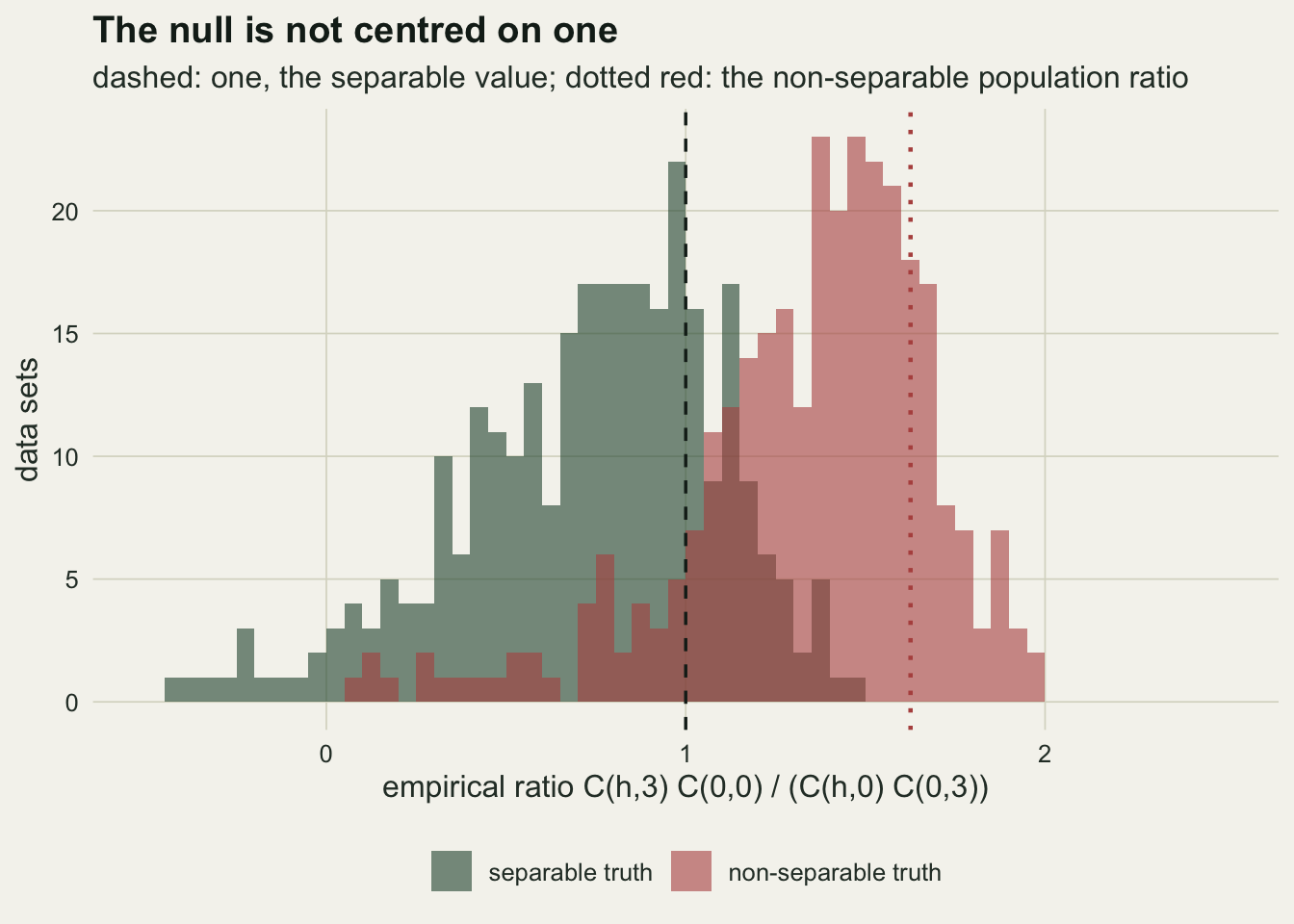
The histogram window runs from -0.5 to 2.5, and 3 of the 600 ratios fall outside it; 15 ratios are negative. In 15 of those the centred lag-three covariance for the band came out below zero, while the lag-three covariance at zero distance stayed at 0.17 or more. Across the separable data sets that numerator has the largest coefficient of variation of the four estimates, 0.73 against at most 0.26 for the other three, which is one more reason not to read the ratio by eye.
What to report
State that the covariance was assumed separable, in those words, and say what it implies for the system: one spatial range at every time lag. For soil moisture, plankton patches, disease incidence or any quantity that diffuses or spreads, that implication is a hypothesis about the ecology, and a reader should be able to see it was made.
Report the fitted spatial range together with the time scale it was estimated alongside, and do not transfer it to another lag without saying so. In the simulation above the separable fit returned a practical range of 6.7 km for data whose true range ran from 9.0 km at lag zero to 18.0 km at six months, and nothing in the fitted parameters warned that this had happened.
If separability is checked, check it against a simulated reference distribution rather than against the value one. Report the band and lag the check used, that they were chosen before looking, and the result as a p value from the bootstrap. A non-rejection with fifty sites and forty times is weak evidence: it failed to detect a strong interaction in more than half of the data sets here.
When the separable model is kept for speed, say how large the computational saving was on the problem in hand, and consider a non-separable fit on a subset of sites as a sensitivity check. A covariance that fits the lag-zero map well can still understate how much one month tells about the next at a neighbouring site.
Honest limits
Only one non-separable family was tried, with one interaction value, one temporal scale and exponential smoothness in space. The Cressie and Huang 1999 construction through spectral densities and other members of the Gneiting class interact differently; a family in which the spatial range shrinks with lag could push the separable fit in another direction, and the direction found here should not be carried over to it.
The non-separable model itself was never fitted. Maximum likelihood for the Gneiting model needs the full Cholesky at every step, and at the timing measured above a few hundred optimiser steps per data set, for three hundred data sets, is out of reach for a page that has to knit. That is the practical argument for separability made concrete, and it also means the post measures what goes wrong with the separable fit rather than how much a correct fit would recover.
The separability test used one distance band and one lag. Pooling several bands and lags, or using a likelihood ratio test of the kind Mitchell, Genton and Gumpertz proposed for replicated data, would be more powerful; the single-band ratio was chosen because it is the check people actually compute. The power figure is for this statistic and this design, not for testing separability in general.
The design is a regular monthly series at fixed sites with no missing values and no measurement error. A nugget that belongs to one factor, as in \(\Sigma_t \otimes (\Sigma_s + \tau^2 I)\), keeps the Kronecker form. Independent measurement error on every reading does not, because it adds \(\tau^2 I\) to the whole matrix and \(\Sigma_t \otimes \Sigma_s + \tau^2 I\) is not a Kronecker product; the eigendecompositions of the two factors still give a fast likelihood, but that is a different algorithm from the one timed here. Genton 2007 discusses approximating a non-separable covariance matrix by the nearest Kronecker product, which is a way of keeping part of the saving while admitting the misfit.
The mean is a single constant. A trend in time or a covariate surface in space would be absorbed through generalised least squares in the same way, but an unmodelled seasonal cycle would leak into the temporal covariance and could imitate or hide an interaction.
References
Gneiting T 2002 Journal of the American Statistical Association 97(458):590-600 (10.1198/016214502760047113)
Cressie N, Huang HC 1999 Journal of the American Statistical Association 94(448):1330-1339 (10.1080/01621459.1999.10473885)
Van Loan CF 2000 Journal of Computational and Applied Mathematics 123(1-2):85-100 (10.1016/S0377-0427(00)00393-9)
Genton MG 2007 Environmetrics 18(7):681-695 (10.1002/env.854)
Mitchell MW, Genton MG, Gumpertz ML 2006 Journal of Multivariate Analysis 97(5):1025-1043 (10.1016/j.jmva.2005.07.005)