library(ggplot2)
library(patchwork)

te_paper  <- "#f5f4ee"
te_ink    <- "#16241d"
te_body   <- "#2c3a31"
te_forest <- "#275139"
te_rust   <- "#b5534e"
te_gold   <- "#c9b458"
te_line   <- "#dad9ca"

theme_datasheet <- function() {
  theme_minimal(base_size = 12) +
    theme(plot.background  = element_rect(fill = te_paper, colour = NA),
          panel.background = element_rect(fill = te_paper, colour = NA),
          panel.grid.major = element_line(colour = te_line, linewidth = 0.3),
          panel.grid.minor = element_blank(),
          text             = element_text(colour = te_body),
          plot.title       = element_text(colour = te_ink, face = "bold"),
          plot.subtitle    = element_text(colour = te_body),
          axis.text        = element_text(colour = te_body),
          strip.text       = element_text(colour = te_ink))
}Sediment quality guidelines from co-occurrence
R
ecotoxicology
sediment quality
logistic regression
simulation
ecology tutorial
At a correlation of 0.8, an inert chemical passes the ERL/ERM reliability check in contaminated databases and the real toxicant fails it in clean ones. R.
An estuary survey programme has a spreadsheet of a few hundred sediment samples. Each row holds the concentrations of a dozen metals and hydrocarbons and the result of an amphipod bioassay: toxic or not. Somebody is asked to turn the spreadsheet into numbers a manager can use, and a method many programmes reach for is the effects range approach of Long and colleagues. Take the samples that were toxic, sort each chemical’s concentrations among them, and read off the 10th percentile as the effects range low (ERL) and the median as the effects range median (ERM). Every chemical in the spreadsheet gets two guideline values, whether or not it had anything to do with the toxicity.
Long, MacDonald, Smith and Calder (1995) did two things with those values, and this post is about the second. After deriving the percentiles from the effects data only, they checked the guidelines by going back to all the samples, effects and no effects alike, and computing the incidence of adverse effects in three ranges: below the ERL, between the two values, and above the ERM. Their paper states no formal pass mark; the text says the incidence of effects “usually was less than 25%” below the ERL and “often” greater than 75% above the ERM, and that for most chemicals it “increased markedly” across the ranges. MacDonald, Ingersoll and Berger (2000) turned the same idea into a rule for their freshwater consensus guidelines: a lower guideline is reliable if more than 75 per cent of the samples below it are correctly predicted to be non-toxic, an upper guideline is reliable if more than 75 per cent of the samples above it are toxic, and the evaluation needs at least 20 samples. That rule, applied to the ERL and the ERM, is the reliability check used below.
The weakness of the recipe is known. O’Connor (2004) argued, in the words of his title, that the ERL is not a chemical concentration at the threshold of sediment toxicity. Field and colleagues (2002) took a different route to guideline values: a logistic regression of amphipod survival test outcome on concentration for each of 37 chemicals, read at fixed probabilities of toxicity, with the single-chemical models then combined through the maximum predicted probability in a sample. Nothing here is a new result. What the simulations add is a measurement of the reliability check itself: whether it can tell a chemical that causes toxicity from one that travels with it, and what it responds to instead.
The problem has relatives elsewhere on this site. Reference sites and tolerance bounds derives a percentile threshold from one clean reference set and one variable, and shows that its false alarm rate belongs to that reference set. Here the percentile is read from a mixed database of toxic and non-toxic samples in which several correlated chemicals are measured at once, so it inherits both the site mix and every chemical that co-varies with the real cause. Co-occurrence is not interaction makes the same kind of point about species that share an unrecorded gradient, and Confounding and backdoor adjustment gives the general regression version. Neither touches a percentile threshold or the check that is supposed to validate one.
The recipe on one simulated database
The simulated world has two chemicals on a standardised log concentration scale. Chemical A is toxic: the probability that a sample fails the bioassay is a logistic curve in A with a slope of 3 per log standard deviation and a midpoint at 1, on top of a background false positive rate of 0.08 that any bioassay has. Chemical B does nothing; it is correlated with A because the two come from the same outfall. Across samples both concentrations are normal with a standard deviation of 1 and a common mean, the database shift, which describes whether the programme sampled mostly clean sites (shift -1), a mixture (0) or mostly contaminated harbours (+1). These constants were fixed before any run and are not tuned anywhere below.
bg_rate   <- 0.08
tox_slope <- 3
tox_mid   <- 1
cut_share <- 0.75
min_n     <- 20

p_toxic <- function(z_a) bg_rate + (1 - bg_rate) * plogis(tox_slope * (z_a - tox_mid))

draw_pair <- function(n, rho, shift) {
  z_a <- rnorm(n, shift)
  z_b <- shift + rho * (z_a - shift) + sqrt(1 - rho^2) * rnorm(n)
  list(z_a = z_a, z_b = z_b, tox = rbinom(n, 1, p_toxic(z_a)))
}

# ERL and ERM: 10th and 50th percentiles among toxic samples (Long et al. 1995)
effects_range <- function(x, tox) quantile(x[tox == 1], c(0.1, 0.5), names = FALSE, type = 7)

# incidence of toxicity below, between and above, on any set of samples
incidence <- function(x, tox, guide) {
  lo <- x < guide[1]; hi <- x > guide[2]; mid <- !lo & !hi
  c(below = mean(tox[lo]), between = mean(tox[mid]), above = mean(tox[hi]),
    n_lo = sum(lo), n_hi = sum(hi))
}

# MacDonald et al. (2000) rule applied to the ERL and the ERM
passes_check <- function(inc) {
  (1 - inc[["below"]]) > cut_share & inc[["above"]] > cut_share &
    inc[["n_lo"]] >= min_n & inc[["n_hi"]] >= min_n
}

n_demo   <- 600
rho_demo <- 0.8
set.seed(4107)
demo_list <- lapply(c(clean = -1, dirty = 1), function(s) {
  d_one <- draw_pair(n_demo, rho_demo, s)
  g_a <- effects_range(d_one$z_a, d_one$tox)
  g_b <- effects_range(d_one$z_b, d_one$tox)
  i_a <- incidence(d_one$z_a, d_one$tox, g_a)
  i_b <- incidence(d_one$z_b, d_one$tox, g_b)
  list(g_a = g_a, g_b = g_b, i_a = i_a, i_b = i_b,
       pass_a = passes_check(i_a), pass_b = passes_check(i_b), prev = mean(d_one$tox))
})
dm_c <- demo_list$clean
dm_d <- demo_list$dirty
Take one database of 600 samples from contaminated harbours (shift +1) with a correlation of 0.8 between the chemicals. 56 per cent of the samples are toxic. The inert chemical B gets an ERL of 0.17 and an ERM of 1.46, and the incidence of toxicity is 26, 49 and 86 per cent below, between and above. That is the pattern Long and colleagues described for a working guideline: low, then middling, then high. Under the 75 per cent rule this particular database misses the lower pass mark by 1.0 percentage points (passes: no); the next section counts how often a database of this kind clears it. The toxic chemical A in the same database shows 16, 63 and 97 per cent and passes (yes). Read as a table of three percentages, both show the rising pattern, and B misses a pass only by that 1.0 percentage points below the ERL.
Now a database of the same size from mostly clean sites (shift -1), with the same toxicity curve. Only 12 per cent of samples are toxic. For A the incidence is 7, 8 and 24 per cent, and the chemical that causes all the toxicity in the simulation fails the check (passes: no). Its ERM is -0.26 against a toxicity midpoint of 1, so most samples above the ERM sit where the bioassay fails only occasionally.
band_levels <- c("below ERL", "between", "above ERM")
demo_df <- do.call(rbind, lapply(names(demo_list), function(nm) {
  dl <- demo_list[[nm]]
  data.frame(database = nm,
             chemical = rep(c("A, toxic", "B, inert"), each = 3),
             band = factor(rep(band_levels, 2), levels = band_levels),
             incidence = c(dl$i_a[1:3], dl$i_b[1:3]))
}))
demo_df$database <- factor(demo_df$database, levels = c("clean", "dirty"),
                           labels = c("clean sites (shift -1)", "contaminated sites (shift +1)"))

ggplot(demo_df, aes(band, incidence, fill = chemical)) +
  geom_col(position = position_dodge(width = 0.75), width = 0.7) +
  geom_hline(yintercept = c(1 - cut_share, cut_share), linetype = "dashed",
             colour = te_rust, linewidth = 0.6) +
  facet_wrap(~ database) +
  scale_fill_manual(values = c(te_forest, te_gold), name = NULL) +
  scale_y_continuous(limits = c(0, 1), breaks = seq(0, 1, 0.25)) +
  labs(x = NULL, y = "share of samples toxic",
       title = "The check reads the database",
       subtitle = "dashed red: pass marks, below ERL under 0.25 and above ERM over 0.75") +
  theme_datasheet() +
  theme(legend.position = "bottom")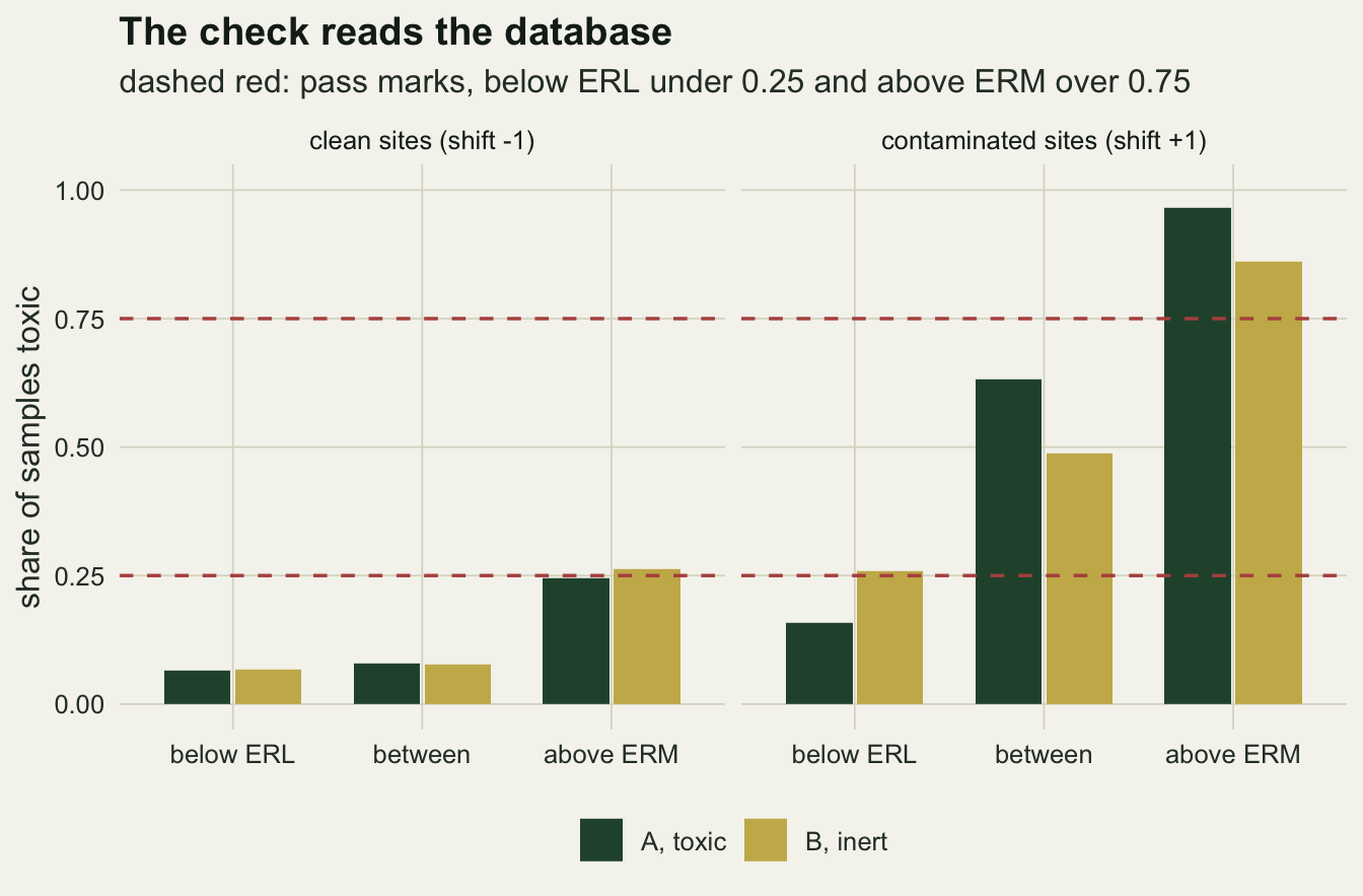
The guideline value is a percentile of a conditional distribution
Before the reliability check, one piece of arithmetic that needs no simulation. Among toxic samples the density of A is the density of A in the database multiplied by the probability of toxicity at each concentration, rescaled. The ERL is the 10th percentile of that product, so it moves with the database mean even though the toxicity curve does not move at all.
shift_grid <- c(-1, 0, 1)
toxic_quantile <- function(shift, prob) {
  dens <- function(z) dnorm(z, shift) * p_toxic(z)
  total <- integrate(dens, -Inf, Inf)$value
  uniroot(function(q) integrate(dens, -Inf, q)$value / total - prob,
          c(shift - 8, shift + 8), tol = 1e-9)$root
}
erl_closed <- sapply(shift_grid, toxic_quantile, prob = 0.1)
erm_closed <- sapply(shift_grid, toxic_quantile, prob = 0.5)
erl_move   <- erl_closed[3] - erl_closed[1]
erl_fold   <- exp(erl_move)
With the toxicity midpoint fixed at 1, the population ERL of A is -2.04, -0.49 and 0.62 for database shifts of -1, 0 and +1, and the ERM is -0.39, 0.96 and 1.57. Moving the database two standard deviations moves the ERL by 2.66 standard deviations; if one standard deviation were one natural log unit of concentration, the ERL would change 14-fold. This is the arithmetic behind O’Connor’s title: at clean sites the toxic samples are mostly background false positives spread over low concentrations, and their 10th percentile is low because the database is.
The reliability check reads the database
The check was run on simulated databases of 150, 600 and 2000 samples, with correlations of 0.3, 0.5 and 0.8 between A and B and the three database shifts: 27 cells with 300 databases each. The unit of the pass rate is the database. Each database was also given a fresh validation set of the same size and make-up, and the check was repeated there with the guidelines from the first set, which is closer to how MacDonald and colleagues evaluated theirs.
wald_p <- function(x_mat, y) {
  fit <- glm.fit(x_mat, y, family = binomial())
  k <- ncol(x_mat)
  cov_b <- chol2inv(fit$qr$qr[1:k, 1:k, drop = FALSE])
  est <- fit$coefficients[fit$qr$pivot]
  p_val <- 2 * pnorm(-abs(est / sqrt(diag(cov_b))))
  p_val[order(fit$qr$pivot)]
}

one_database <- function(n, rho, shift) {
  d_tr <- draw_pair(n, rho, shift)
  d_va <- draw_pair(n, rho, shift)
  g_a <- effects_range(d_tr$z_a, d_tr$tox)
  g_b <- effects_range(d_tr$z_b, d_tr$tox)
  i_a <- incidence(d_tr$z_a, d_tr$tox, g_a)
  i_b <- incidence(d_tr$z_b, d_tr$tox, g_b)
  p_uni   <- wald_p(cbind(1, d_tr$z_b), d_tr$tox)[2]
  p_joint <- wald_p(cbind(1, d_tr$z_a, d_tr$z_b), d_tr$tox)
  c(erl_a = g_a[1], above_a = i_a[["above"]], below_a = i_a[["below"]],
    above_b = i_b[["above"]], below_b = i_b[["below"]],
    pass_a = passes_check(i_a), pass_b = passes_check(i_b),
    val_a = passes_check(incidence(d_va$z_a, d_va$tox, g_a)),
    val_b = passes_check(incidence(d_va$z_b, d_va$tox, g_b)),
    loose_a = i_a[["below"]] < 0.25 & i_a[["above"]] >= 0.5 & i_a[["n_lo"]] >= min_n & i_a[["n_hi"]] >= min_n,
    loose_b = i_b[["below"]] < 0.25 & i_b[["above"]] >= 0.5 & i_b[["n_lo"]] >= min_n & i_b[["n_hi"]] >= min_n,
    uni_b = p_uni < 0.05, joint_a = p_joint[2] < 0.05, joint_b = p_joint[3] < 0.05)
}

n_rep <- 300
cells <- expand.grid(n = c(150, 600, 2000), rho = c(0.3, 0.5, 0.8), shift = shift_grid)
set.seed(20260918)
grid_tab <- cbind(cells, t(sapply(seq_len(nrow(cells)), function(i) {
  rowMeans(replicate(n_rep, one_database(cells$n[i], cells$rho[i], cells$shift[i])),
           na.rm = TRUE)
})))

cell <- function(n, rho, shift, col) grid_tab[grid_tab$n == n & grid_tab$rho == rho &
                                              grid_tab$shift == shift, col]
mcse <- function(p) sqrt(p * (1 - p) / n_rep)

erl_sim_max_gap <- max(abs(sapply(seq_along(shift_grid), function(j)
  cell(2000, 0.8, shift_grid[j], "erl_a") - erl_closed[j])))
pass_a_clean_max <- max(grid_tab$pass_a[grid_tab$shift == -1])
above_a_clean <- range(grid_tab$above_a[grid_tab$shift == -1])
pass_a_mid    <- range(grid_tab$pass_a[grid_tab$shift == 0])
pass_a_dirty  <- range(grid_tab$pass_a[grid_tab$shift == 1])
pass_b_dirty8 <- sapply(c(150, 600, 2000), function(n) cell(n, 0.8, 1, "pass_b"))
pass_b_low    <- max(grid_tab$pass_b[grid_tab$rho < 0.8])
pass_b_mid8   <- max(grid_tab$pass_b[grid_tab$rho == 0.8 & grid_tab$shift < 1])
above_b_dirty8 <- cell(2000, 0.8, 1, "above_b")
below_b_dirty8 <- cell(2000, 0.8, 1, "below_b")
val_b_dirty8  <- sapply(c(150, 600, 2000), function(n) cell(n, 0.8, 1, "val_b"))
val_a_clean_max <- max(grid_tab$val_a[grid_tab$shift == -1])
val_gap_all   <- pmax(abs(grid_tab$val_a - grid_tab$pass_a), abs(grid_tab$val_b - grid_tab$pass_b))
val_gap_max   <- max(val_gap_all)
val_gap_big   <- max(val_gap_all[grid_tab$n >= 600])
val_gap_n     <- grid_tab$n[which.max(val_gap_all)]
loose_b_mid8  <- sapply(c(150, 600, 2000), function(n) cell(n, 0.8, 0, "loose_b"))
loose_b_dirty8 <- sapply(c(150, 600, 2000), function(n) cell(n, 0.8, 1, "loose_b"))
loose_a_clean_max <- max(grid_tab$loose_a[grid_tab$shift == -1])
The simulated mean ERL of A at 2000 samples and a correlation of 0.8 sits within 0.023 log units of the closed form at all three shifts, so the arithmetic above and the simulation agree.
In databases from clean sites the toxic chemical never passed: its highest pass rate in any of the nine clean cells is 0.000 of 300 databases, because the incidence of toxicity above its ERM averages only 0.22 to 0.25. In mixed databases it passed in 0.44 to 0.75 of databases, and in contaminated ones in 0.99 to 1.00. The chemical and its toxicity curve are the same in all 27 cells.
The inert chemical fails where the toxic one passes, except in one corner. At correlations of 0.3 and 0.5 it essentially never passed (at most 0.037 of databases in any cell), and at 0.8 it failed in clean and mixed databases (at most 0.057). In contaminated databases with a correlation of 0.8 it passed in 0.66, 0.96 and 1.00 of databases of 150, 600 and 2000 samples (Monte Carlo standard error at most 0.027). With 2000 samples its average incidence was 0.21 below the ERL and 0.84 above the ERM. More data did not make the check more discerning; it made the wrong verdict more certain.
Scoring the guidelines on an independent validation set did not change the picture. Across all 27 cells and both chemicals the pass rate moved by at most 0.17, in a cell with 150 samples, and by at most 0.08 with 600 or more; the inert chemical still passed in 0.61 to 0.98 of contaminated databases at a correlation of 0.8, and the toxic one passed in none of the clean ones. Independent data guard against overfitting. They do not guard against a validation set with the same site mix and the same correlations, which is what any second sample from the same programme will have.
pass_long <- rbind(
  data.frame(grid_tab[, c("n", "rho", "shift")], chemical = "A, toxic", pass = grid_tab$pass_a),
  data.frame(grid_tab[, c("n", "rho", "shift")], chemical = "B, inert", pass = grid_tab$pass_b))
pass_long$rho_lab <- factor(paste("correlation", pass_long$rho))
pass_long$size    <- factor(pass_long$n, levels = c(150, 600, 2000))

ggplot(pass_long, aes(shift, pass, colour = chemical, linetype = size, group = interaction(chemical, size))) +
  geom_line(linewidth = 0.8) +
  geom_point(aes(shape = size), size = 2) +
  facet_wrap(~ rho_lab) +
  scale_colour_manual(values = c(te_forest, te_gold), name = NULL) +
  scale_x_continuous(breaks = shift_grid, labels = c("clean", "mixed", "dirty")) +
  labs(x = "database make-up (shift in log sd)", y = "share of databases passing",
       linetype = "samples", shape = "samples",
       title = "The site mix decides the verdict at the extremes",
       subtitle = "300 databases per point; toxicity depends on A only") +
  theme_datasheet() +
  theme(legend.position = "bottom", legend.box = "horizontal",
        panel.spacing = unit(1.2, "lines"))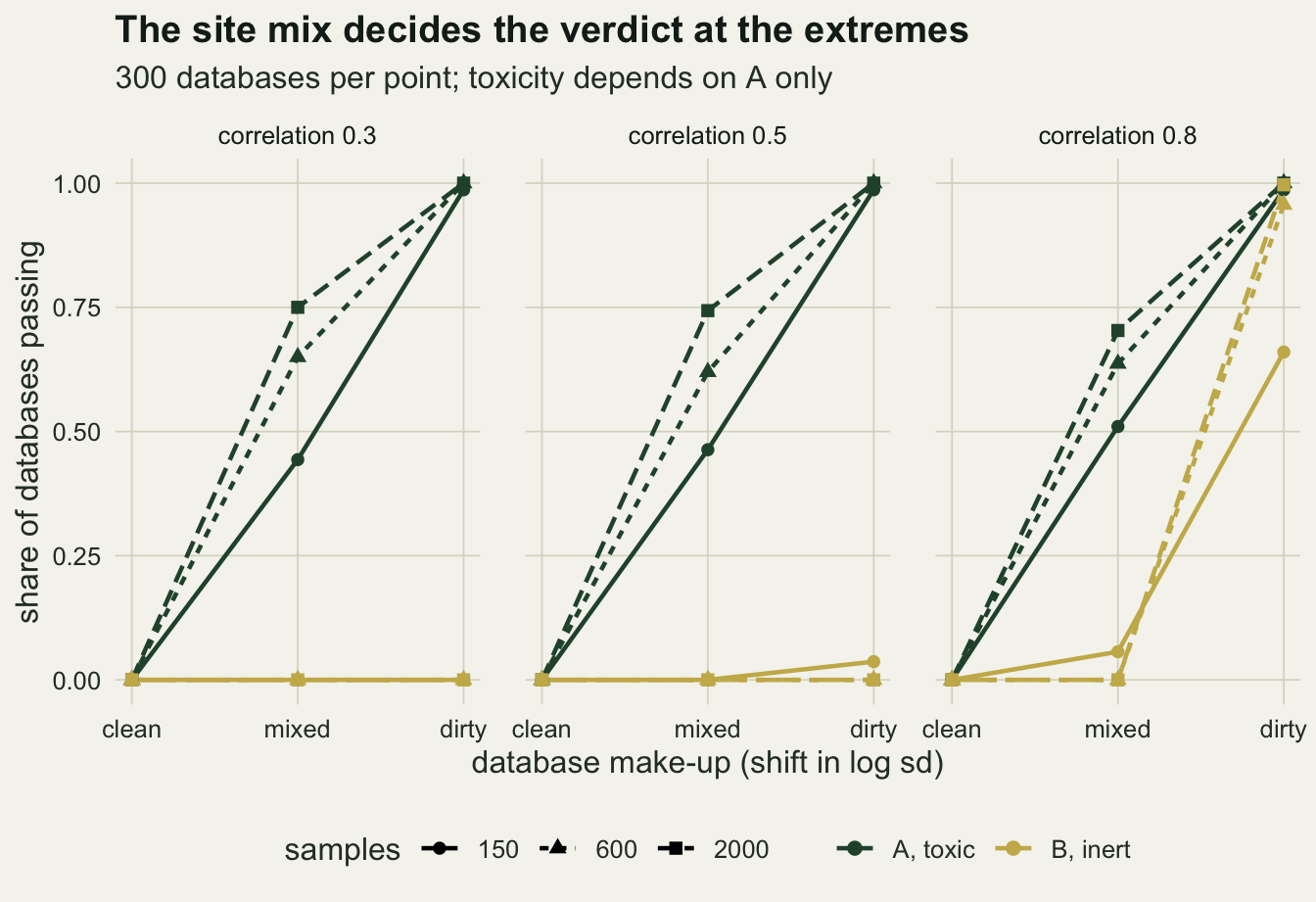
A regression on one chemical at a time
Field and colleagues replaced the percentiles with a logistic regression of the bioassay outcome on each chemical’s concentration. That uses every sample, but it still asks one chemical at a time whether toxicity rises with its concentration, and it answers yes for the inert chemical far more readily than the 75 per cent check does: with 600 samples, a correlation of 0.5 and a mixed database, it called B significant in 1.00 of databases, and the check passed B in 0.000. A joint model with both chemicals asks whether B adds anything once A is known. The same 300 databases per cell were fitted both ways, with a Wald test at the five per cent level.
uni_b_8   <- sapply(shift_grid, function(s) cell(600, 0.8, s, "uni_b"))
uni_b_3   <- sapply(shift_grid, function(s) cell(600, 0.3, s, "uni_b"))
joint_b_rng <- range(grid_tab$joint_b)
joint_b_mean <- mean(grid_tab$joint_b)
joint_a_150 <- cell(150, 0.8, -1, "joint_a")
joint_a_600 <- range(grid_tab$joint_a[grid_tab$n == 600])
joint_a_2000 <- min(grid_tab$joint_a[grid_tab$n == 2000])
uni_b_3_big <- cell(2000, 0.3, -1, "uni_b")
With 600 samples and a correlation of 0.8, the one-chemical logistic called the inert B significant in 0.97, 1.00 and 1.00 of clean, mixed and contaminated databases; even at a correlation of 0.3 the rates were 0.37, 0.96 and 0.99. The site mix changes these rates mainly through how much information the database carries about the toxicity curve; the error itself comes from the correlation, and with more samples a weaker correlation is enough: at 2000 samples and a correlation of 0.3 the rate in clean databases was 0.84.
The joint model flagged B in between 0.027 and 0.070 of databases across the 27 cells, with a mean of 0.048; the Monte Carlo standard error at a true rate of 0.05 is 0.013, so the rates are consistent with the nominal five per cent. It found A in 0.88 to 1.00 of databases of 600 samples and in every database at 2000, but only 0.34 with 150 samples from clean sites and a correlation of 0.8, where there are few toxic samples and A and B carry nearly the same information.
sub8 <- grid_tab[grid_tab$rho == 0.8, ]
logit_long <- rbind(
  data.frame(sub8[, c("n", "shift")], test = "B, one-chemical model", rate = sub8$uni_b),
  data.frame(sub8[, c("n", "shift")], test = "B, joint model", rate = sub8$joint_b),
  data.frame(sub8[, c("n", "shift")], test = "A, joint model", rate = sub8$joint_a))
logit_long$shift_lab <- factor(logit_long$shift, levels = shift_grid,
                               labels = c("clean sites", "mixed", "contaminated sites"))

ggplot(logit_long, aes(n, rate, colour = test)) +
  geom_hline(yintercept = 0.05, linetype = "dashed", colour = te_rust, linewidth = 0.6) +
  geom_line(linewidth = 0.8) +
  geom_point(size = 2) +
  facet_wrap(~ shift_lab) +
  scale_x_log10(breaks = c(150, 600, 2000)) +
  scale_colour_manual(values = c(te_forest, te_ink, te_gold), name = NULL) +
  scale_y_continuous(limits = c(0, 1)) +
  labs(x = "samples in the database (log scale)", y = "share of databases with p < 0.05",
       title = "Only the joint model lets the inert chemical go",
       subtitle = "dashed red: the nominal five per cent") +
  theme_datasheet() +
  theme(legend.position = "bottom", panel.spacing = unit(1.2, "lines"))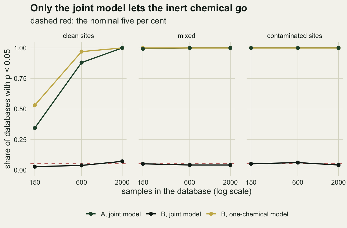
When toxicity is not a logistic in one analyte
The joint model above was fitted in the form the data were simulated from, which is generous. Real toxicity may switch on at a threshold, or come from a mixture in which each chemical contributes toxic units. A third chemical C was added, correlated 0.8 with B and so 0.64 with A, which puts B in the middle of the correlation structure. Four worlds were simulated at database shifts of 0 and +1 with 600 and 2000 samples: toxicity logistic in A as before; a step in A, with a toxic probability of 0.85 above the midpoint and the background below it; toxic units from A and C together, with C measured and in the model; and the same toxic unit mixture with C never measured. In every world B is inert.
draw_three <- function(n, shift, form) {
  z_b <- rnorm(n, shift)
  z_a <- shift + 0.8 * (z_b - shift) + 0.6 * rnorm(n)
  z_c <- shift + 0.8 * (z_b - shift) + 0.6 * rnorm(n)
  p_t <- switch(form,
                logistic = p_toxic(z_a),
                step     = ifelse(z_a > tox_mid, 0.85, bg_rate),
                bg_rate + (1 - bg_rate) * plogis(tox_slope * (log(exp(z_a) + exp(z_c)) - 1.5)))
  list(z_a = z_a, z_b = z_b, z_c = z_c, tox = rbinom(n, 1, p_t))
}
arm_one <- function(n, shift, form) {
  d_m <- draw_three(n, shift, form)
  x_mat <- if (form == "units, C unmeasured") cbind(1, d_m$z_a, d_m$z_b) else
    cbind(1, d_m$z_a, d_m$z_b, d_m$z_c)
  p_val <- wald_p(x_mat, d_m$tox)
  c(flag_b = p_val[3] < 0.05, flag_a = p_val[2] < 0.05,
    pass_b = passes_check(incidence(d_m$z_b, d_m$tox, effects_range(d_m$z_b, d_m$tox))))
}
form_levels <- c("logistic in A", "step in A", "units, C measured", "units, C unmeasured")
arm_cells <- expand.grid(form = form_levels, n = c(600, 2000), shift = c(0, 1),
                         stringsAsFactors = FALSE)
arm_key <- c("logistic in A" = "logistic", "step in A" = "step",
             "units, C measured" = "units", "units, C unmeasured" = "units, C unmeasured")
set.seed(918)
arm_tab <- cbind(arm_cells, t(sapply(seq_len(nrow(arm_cells)), function(i) {
  rowMeans(replicate(n_rep, arm_one(arm_cells$n[i], arm_cells$shift[i],
                                    arm_key[[arm_cells$form[i]]])))
})))
arm_rate <- function(form, col) arm_tab[arm_tab$form == form, col]
step_b   <- range(arm_rate("step in A", "flag_b"))
unitm_b  <- range(arm_rate("units, C measured", "flag_b"))
logit_b  <- range(arm_rate("logistic in A", "flag_b"))
unitu_b  <- range(arm_rate("units, C unmeasured", "flag_b"))
arm_a_min <- min(arm_tab$flag_a)
arm_z_max <- max((arm_tab$flag_b[arm_tab$form != "units, C unmeasured"] - 0.05) / mcse(0.05))
arm_pass_b_dirty <- arm_tab[arm_tab$shift == 1 & arm_tab$n == 2000, c("form", "pass_b")]
The shape of the toxicity curve troubled the joint model little. With a step in A it flagged B in 0.020 to 0.037 of databases across the four cells, and with a toxic unit mixture in which C was in the model, in 0.043 to 0.077, against 0.040 to 0.050 when the model form was right. The largest of these rates is 2.1 Monte Carlo standard errors above 0.05. A itself was found in every database of every world. The reason is structural rather than lucky: when toxicity depends on measured chemicals only, B carries no information once those chemicals are in the model, whatever the curve looks like, and a misfitted curve has nothing to borrow from B.
Leave C out, and B becomes its stand-in. With the mixture toxic through A and an unmeasured C, the joint model flagged the inert B in 0.973 to 1.000 of databases. The joint model separates a cause from a co-travelling chemical only among the chemicals that were measured; it cannot separate a measured chemical from an unmeasured toxicant it is correlated with, and in a real sediment the list of unmeasured compounds is long. The 75 per cent check gives no help here either: in contaminated databases of 2000 samples it passed the inert B in 0.997 of databases when toxicity was logistic in A, 0.883 with a step, and 0.487 and 0.487 in the two toxic unit worlds.
arm_tab$form_f <- factor(arm_tab$form, levels = rev(form_levels))
arm_tab$setting <- paste0(arm_tab$n, " samples, ", ifelse(arm_tab$shift == 0, "mixed", "contaminated"))

ggplot(arm_tab, aes(flag_b, form_f, colour = setting, shape = setting)) +
  geom_vline(xintercept = 0.05, linetype = "dashed", colour = te_rust, linewidth = 0.6) +
  geom_point(size = 2.8, position = position_dodge(width = 0.5)) +
  scale_colour_manual(values = c(te_forest, te_gold, te_ink, te_rust), name = NULL) +
  scale_shape_manual(values = c(16, 17, 15, 18), name = NULL) +
  scale_x_continuous(limits = c(0, 1)) +
  labs(x = "share of databases flagging inert B (p < 0.05)", y = NULL,
       title = "The joint model fails only on what was not measured",
       subtitle = "dashed red: the nominal five per cent; 300 databases per point") +
  guides(colour = guide_legend(nrow = 2), shape = guide_legend(nrow = 2)) +
  theme_datasheet() +
  theme(legend.position = "bottom")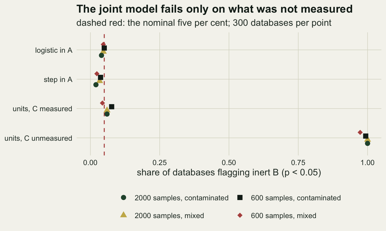
What to report
Report ERL and ERM values as descriptions of the database they came from, with its size, the share of toxic samples and a sentence on the site mix. The same toxicity curve gave an ERL of -2.04 or 0.62 depending only on whether the sites were mostly clean or mostly contaminated, so a guideline without that context cannot be compared with one from another programme.
Do not present a pass on the incidence check as evidence that a chemical causes toxicity. In the simulation a chemical with no effect passed in most contaminated databases when its correlation with the real toxicant was 0.8, and the real toxicant failed in every clean database. The check measures how well a chemical sorts toxic from non-toxic samples in that database, which is useful for screening and says nothing about which chemical to regulate or remediate.
If the question is which chemicals matter, fit the chemicals together and report the correlation matrix of the log concentrations beside the model. The joint logistic regression stayed near its nominal error rate for an inert chemical under three different toxicity mechanisms. State which chemicals were not measured, because an unmeasured co-sourced toxicant turns an inert measured chemical into a significant one, and no model on the measured list can detect that.
Honest limits
The simulated databases are far tidier than the ones Long and colleagues assembled. Their database pooled field surveys, spiked laboratory tests and equilibrium partitioning values from many species and endpoints, screened each entry for concordance, and treated a small gradient or no gradient as a no-effects entry. Here there is one bioassay with a fixed false positive rate of 0.08 and one toxic mechanism, so the numbers above show the direction and the rough size of the problem for the recipe, not the error rate of any published guideline.
The pass rule is MacDonald and colleagues’ 75 per cent rule for their consensus TECs and PECs, applied here to the ERL and the ERM. Long and colleagues gave no formal rule. A looser reading, under 25 per cent below the ERL and at least 50 per cent above the ERM, was also scored in the same databases: at a correlation of 0.8 the inert chemical then passed in 0.66, 0.83 and 0.92 of mixed databases of 150, 600 and 2000 samples and in 0.73 to 1.00 of contaminated ones, while the toxic chemical passed in at most 0.01 of clean databases. The looser the rule, the more often the inert chemical passes. Current practice also leans on consensus guidelines, the geometric mean of several guideline values, and on mean quotients across chemicals; neither was simulated. A consensus value averages guidelines that each inherit the same database and the same correlations, so there is no reason to expect it to remove the effect, but that is an expectation and not a measurement.
The correlation of 0.8 is the setting in which the inert chemical passed. Metals delivered by the same effluent, or hydrocarbons from the same combustion source, can be that strongly correlated on the log scale, and fine-grained, organic-rich sediment raises many contaminants together; but whether a given pair is correlated that strongly is a property of the survey, and at 0.5 the inert chemical almost never passed. The concentrations are normal on the log scale with equal variances, which real sediment data are not.
The joint model was given the right chemicals except in the one arm built to show what happens without them. With a dozen or more correlated analytes and a few hundred samples, the joint model has its own problems: separation, unstable coefficients and a multiplicity of tests that the single Wald test here does not face. The model comparison says a joint model is the right question to ask, not that it will answer it cleanly with a real database.
References
Long ER, MacDonald DD, Smith SL, Calder FD 1995 Environmental Management 19(1):81-97 (10.1007/BF02472006)
MacDonald DD, Ingersoll CG, Berger TA 2000 Archives of Environmental Contamination and Toxicology 39(1):20-31 (10.1007/s002440010075)
Field LJ, MacDonald DD, Norton SB, Ingersoll CG, Severn CG, Smorong D, Lindskoog R 2002 Environmental Toxicology and Chemistry 21(9):1993-2005 (10.1002/etc.5620210929)
O’Connor TP 2004 Marine Pollution Bulletin 49(5-6):383-385 (10.1016/j.marpolbul.2004.06.024)