library(ggplot2)
library(patchwork)

te_paper  <- "#f5f4ee"
te_ink    <- "#16241d"
te_body   <- "#2c3a31"
te_forest <- "#275139"
te_rust   <- "#b5534e"
te_gold   <- "#c9b458"
te_line   <- "#dad9ca"

theme_datasheet <- function() {
  theme_minimal(base_size = 12) +
    theme(plot.background  = element_rect(fill = te_paper, colour = NA),
          panel.background = element_rect(fill = te_paper, colour = NA),
          panel.grid.major = element_line(colour = te_line, linewidth = 0.3),
          panel.grid.minor = element_blank(),
          text             = element_text(colour = te_body),
          plot.title       = element_text(colour = te_ink, face = "bold"),
          plot.subtitle    = element_text(colour = te_body),
          axis.text        = element_text(colour = te_body))
}Runs of homozygosity and realised inbreeding
R
population genetics
inbreeding
conservation genetics
simulation
ecology tutorial
Simulate a linked genome in R and score runs of homozygosity, SNP homozygosity and pedigree F against the realised inbreeding they are meant to measure.
A reintroduced herd has been kept as a closed population for ten generations. Every animal has parents in the studbook, so every animal has an inbreeding coefficient, and the management plan is built on those numbers: pairs above a threshold are not put together, and the mean coefficient of the herd is the figure that goes into the annual report. This year the programme also has a SNP panel on every living animal, and the first question in the meeting is whether the panel says anything the studbook did not.
The studbook coefficient is an expectation. It is the probability that the two alleles an animal carries at a locus picked at random are copies of the same founder allele, averaged over every way the meiotic dice could have fallen. The animal itself got one throw of those dice. Two full sibs have the same pedigree coefficient by construction, and they do not have the same genome: one may have inherited twice as much identical material as the other. That difference is what a dense marker panel can see and a studbook cannot, and it exists only because chromosomes are inherited in segments rather than locus by locus.
This site has been here before and stopped at the door. The post on heterozygosity-fitness correlations simulates unlinked microsatellites, and its honest limits say in as many words that real genomes are linked, that realised inbreeding varies around pedigree f through Mendelian sampling of chromosome segments, and that the case was left out because it needs a linkage model to be honest. This post builds that linkage model. Once segments exist, a homozygous stretch of markers is a read-out of one segment of shared ancestry, and the keyhole becomes a window.
It also inverts the role linkage plays elsewhere here. In checking an effective size estimate physical linkage is a nuisance: it adds association between markers that persists across generations, inflates the mean squared correlation and deflates the estimate of effective size. Here linkage is the entire signal, because without it there would be no runs to find. And in the pedigree posts, the animal model, checking an animal model and mean kinship breeding, the pedigree inbreeding coefficient is taken as given and, implicitly, as the truth; the last of those manages mean kinship and is explicit that inbreeding is a different target. In this simulation the pedigree coefficient is not the truth. The founder labels are.
The ranking that comes out is not a new result. Keller, Visscher and Goddard (2011) showed on simulated dense SNP data that a run-based coefficient predicts realised inbreeding better than the pedigree does, and Kardos, Luikart and Allendorf (2015) made the same case for wild populations with the pedigrees that conservation genetics actually has. What is measured here, and what the post is built around, is the surface underneath that ranking: how the correlation and the false-run share move together across SNP density and minimum run length, with the spread across replicate genomes shown rather than one lucky cell.
Building a genome that knows where its segments came from
n_ind    <- 80          # animals per generation
n_gen    <- 10          # generations of closed breeding
n_rep    <- 8           # replicate genomes
dens_set <- c(1, 5, 20) # SNPs per centimorgan
min_set  <- c(1, 2, 5, 10)  # minimum run length, centimorgans
beta_sh  <- 0.5         # founder frequency spectrum, beta(0.5, 0.5)
chance_hom_cf <- 1 - 2 * (beta_sh / (2 * beta_sh) -
  (beta_sh * (beta_sh + 1)) / ((2 * beta_sh) * (2 * beta_sh + 1)))
n_ped_row <- n_ind * (n_gen + 1)
The population is 80 animals, closed, mating at random without selfing, for ten discrete generations. The genome is five chromosomes of one hundred centimorgans, a map of five morgans in total. That is short for a vertebrate, perhaps a seventh of a real one, and the last section measures what the shortness costs the pedigree. Every founder haplotype carries a label, from one to twice the population size, and every position in every gamete carries the label of the founder haplotype it descends from. Recombination moves labels around: each chromosome gets a Poisson number of crossovers with mean equal to its length in morgans, the crossover positions are uniform, and findInterval decides which parental haplotype each marker copies from.
Realised inbreeding is then exact and needs no estimation. It is the share of positions at which an animal’s two labels are the same. Pedigree inbreeding comes from the tabular method on the same pedigree, and the SNP genotypes come from founder allele frequencies drawn from a beta distribution with both shape parameters at one half, which is the U-shaped spectrum a SNP panel ascertained in another population tends to give. Founders carry no linkage disequilibrium, which matters later.
Under that spectrum the expected homozygosity at a position where the two alleles are not identical by descent is 0.75 in closed form, because the beta with both parameters one half has a mean of one half and a second moment of three eighths, so the expected heterozygosity is one quarter. That single number is why low density panels behave as badly as they do below.
make_ped <- function(n_ind, n_gen) {
  lapply(seq_len(n_gen), function(g) {
    sire <- sample(n_ind, n_ind, replace = TRUE)
    dam  <- vapply(sire, function(x) sample(setdiff(seq_len(n_ind), x), 1), 1L)
    cbind(sire = sire, dam = dam)
  })
}

ped_f <- function(mate, n_ind, n_gen) {
  ped <- data.frame(sire = rep(0L, n_ind), dam = rep(0L, n_ind))
  for (g in seq_len(n_gen))
    ped <- rbind(ped, data.frame(sire = (g - 1) * n_ind + mate[[g]][, "sire"],
                                 dam  = (g - 1) * n_ind + mate[[g]][, "dam"]))
  n_p  <- nrow(ped)
  amat <- matrix(0, n_p, n_p)
  for (i in seq_len(n_p)) {
    si <- ped$sire[i]; di <- ped$dam[i]
    if (si > 0) {
      amat[i, 1:(i - 1)] <- 0.5 * (amat[si, 1:(i - 1)] + amat[di, 1:(i - 1)])
      amat[1:(i - 1), i] <- amat[i, 1:(i - 1)]
      amat[i, i] <- 1 + 0.5 * amat[si, di]
    } else amat[i, i] <- 1
  }
  diag(amat)[(n_gen * n_ind) + seq_len(n_ind)] - 1
}

make_pop <- function(dens, mate, n_chr = 5, chr_len = 100, ld_cm = 0, n_anc = 8) {
  n_pos <- round(chr_len * dens)
  posn  <- (seq_len(n_pos) - 0.5) / dens
  n_tot <- n_chr * n_pos
  pfreq <- rbeta(n_tot, beta_sh, beta_sh)
  if (ld_cm <= 0) {
    fall <- matrix(rbinom(2 * n_ind * n_tot, 1, rep(pfreq, each = 2 * n_ind)),
                   2 * n_ind, n_tot)
    copy <- NULL                              # each founder is its own ancestor
  } else {
    anc  <- matrix(rbinom(n_anc * n_tot, 1, rep(pfreq, each = n_anc)), n_anc, n_tot)
    gapv <- rep(1 / dens, n_tot)
    gapv[seq(1, n_tot, by = n_pos)] <- Inf     # chromosome starts are free
    swp  <- matrix(runif(2 * n_ind * n_tot) < rep(1 - exp(-gapv / ld_cm),
                   each = 2 * n_ind), 2 * n_ind, n_tot)
    copy <- matrix(0L, 2 * n_ind, n_tot)
    for (h in seq_len(2 * n_ind)) {
      seg <- cumsum(swp[h, ])
      copy[h, ] <- sample.int(n_anc, max(seg) + 1L, replace = TRUE)[seg + 1L]
    }
    fall <- matrix(anc[cbind(as.vector(copy), rep(seq_len(n_tot), each = 2 * n_ind))],
                   2 * n_ind, n_tot)
  }
  lab <- list(matrix(rep(seq_len(n_ind), n_tot), n_ind, n_tot),
              matrix(rep(n_ind + seq_len(n_ind), n_tot), n_ind, n_tot))
  lam <- chr_len / 100
  recomb <- function(h1, h2) {
    out <- h1
    for (cc in seq_len(n_chr)) {
      idx  <- (cc - 1) * n_pos + seq_len(n_pos)
      cros <- sort(runif(rpois(1, lam), 0, chr_len))
      take <- (findInterval(posn, cros) + rbinom(1, 1, 0.5)) %% 2 == 1
      out[idx[take]] <- h2[idx[take]]
    }
    out
  }
  for (g in seq_len(n_gen)) {
    si <- mate[[g]][, "sire"]; di <- mate[[g]][, "dam"]
    g1 <- t(vapply(seq_len(n_ind),
                   function(i) recomb(lab[[1]][si[i], ], lab[[2]][si[i], ]),
                   numeric(n_tot)))
    g2 <- t(vapply(seq_len(n_ind),
                   function(i) recomb(lab[[1]][di[i], ], lab[[2]][di[i], ]),
                   numeric(n_tot)))
    lab <- list(g1, g2)
  }
  ibd  <- lab[[1]] == lab[[2]]
  jj   <- rep(seq_len(n_tot), each = n_ind)
  al1  <- fall[cbind(as.vector(lab[[1]]), jj)]
  al2  <- fall[cbind(as.vector(lab[[2]]), jj)]
  anc_ibd <- if (is.null(copy)) ibd else
    matrix(copy[cbind(as.vector(lab[[1]]), jj)] ==
           copy[cbind(as.vector(lab[[2]]), jj)], n_ind, n_tot)
  dose <- matrix(al1 + al2, n_ind, n_tot)
  list(hom = dose != 1L, ibd = ibd, anc_ibd = anc_ibd, dose = dose,
       f_real = rowMeans(ibd), f_anc = rowMeans(anc_ibd),
       n_pos = n_pos, n_chr = n_chr, dens = dens, chr_len = chr_len,
       p_base = colMeans(fall))
}
The run caller is the plain one: a run is a stretch of consecutive homozygous calls on one chromosome, and it is called if it is at least the minimum length. Written with the positions of the heterozygous calls as breakpoints it also gives the lenient caller for free, by allowing a fixed number of heterozygous sites inside a run.
roh_scan <- function(pop, min_cm, max_het = 0) {
  n_pos    <- pop$n_pos
  min_snp  <- min_cm * pop$dens
  win_step <- max_het + 1L
  t(vapply(seq_len(nrow(pop$hom)), function(i) {
    inrun <- logical(ncol(pop$hom))
    for (cc in seq_len(pop$n_chr)) {
      idx <- (cc - 1) * n_pos + seq_len(n_pos)
      brk <- c(0L, which(!pop$hom[i, idx]), n_pos + 1L)
      nb  <- length(brk)
      if (nb <= win_step) next
      lo   <- brk[seq_len(nb - win_step)] + 1L
      hi   <- brk[seq_len(nb - win_step) + win_step] - 1L
      keep <- (hi - lo + 1L) >= min_snp
      if (!any(keep)) next
      dvec <- integer(n_pos + 1L)
      dvec[lo[keep]]     <- dvec[lo[keep]] + 1L
      dvec[hi[keep] + 1L] <- dvec[hi[keep] + 1L] - 1L
      inrun[idx] <- cumsum(dvec)[seq_len(n_pos)] > 0L
    }
    c(froh  = mean(inrun),
      false = if (any(inrun)) mean(!pop$ibd[i, inrun]) else NA_real_,
      only  = if (any(inrun)) mean(!pop$anc_ibd[i, inrun]) else NA_real_)
  }, numeric(3)))
}

safe_cor <- function(x, y) if (sd(x) == 0 || sd(y) == 0) NA_real_ else cor(x, y)

f_excess <- function(pop, base = TRUE) {
  pv    <- if (base) pop$p_base else colMeans(pop$dose) / 2
  e_hom <- sum(pv^2 + (1 - pv)^2)
  (rowSums(pop$hom) - e_hom) / (ncol(pop$hom) - e_hom)
}set.seed(20260920)
mate_one <- make_ped(n_ind, n_gen)
fped_one <- ped_f(mate_one, n_ind, n_gen)
pop_one <- make_pop(5, mate_one)
f_real_one <- pop_one$f_real
slope_one <- coef(lm(f_real_one ~ fped_one))[2]
cor_one <- cor(fped_one, f_real_one)
exc_base_1 <- mean(f_excess(pop_one))
exc_samp_1 <- mean(f_excess(pop_one, base = FALSE))
mean_ped <- mean(fped_one)
mean_real <- mean(f_real_one)
sd_ped <- sd(fped_one)
sd_real <- sd(f_real_one)
sd_dev <- sd(f_real_one - fped_one)
chance_hom <- mean(pop_one$hom[!pop_one$ibd])
chance_gap <- abs(chance_hom - chance_hom_cf)
band <- abs(fped_one - mean_ped) < 0.005
band_lo <- min(f_real_one[band]); band_hi <- max(f_real_one[band])
band_n <- sum(band)The pedigree has 880 rows and the last generation has 80 animals. In this one simulated herd their mean pedigree coefficient is 0.058 and their mean realised inbreeding is 0.053. Whether the pedigree is unbiased for the mean is a claim about the average over herds, not about this one, and the next section tests it on eight.
What one herd does show is the individual scatter. The standard deviation of the pedigree coefficient across these animals is 0.034, while the standard deviation of realised inbreeding is 0.043, and the deviation of one from the other has a standard deviation of 0.041. The correlation between them is 0.46. Among the 7 animals whose pedigree coefficients sit within five thousandths of the herd mean, realised inbreeding runs from 0.013 to 0.098. The least squares line through the scatter has a slope of 0.58 rather than one, which is itself a warning about reading a single population: eight of them put that slope back where theory says it belongs. Hill and Weir (2011) worked out how the scatter depends on genome length and chromosome number; the last section measures the direction of their prediction here.
The arithmetic check for the marker side comes out as expected too. Among positions that are not identical by descent, the share of animals homozygous anyway is 0.750, against the closed form 0.750 for this founder spectrum, a gap of 0.0002. Three quarters of the genome looks homozygous for reasons that have nothing to do with inbreeding, and any run caller has to see past that.
scat_df <- data.frame(f_ped = fped_one, f_real = f_real_one)

ggplot(scat_df, aes(f_ped, f_real)) +
  geom_abline(slope = 1, intercept = 0, linetype = "dashed",
              colour = te_body, linewidth = 0.6) +
  geom_point(colour = te_forest, size = 2, alpha = 0.85) +
  geom_smooth(method = "lm", formula = y ~ x, se = FALSE,
              colour = te_rust, linewidth = 0.8) +
  labs(x = "pedigree inbreeding coefficient",
       y = "realised inbreeding (share of genome identical by descent)",
       title = "One pedigree coefficient, many genomes",
       subtitle = "dashed: one to one; red: least squares fit") +
  theme_datasheet()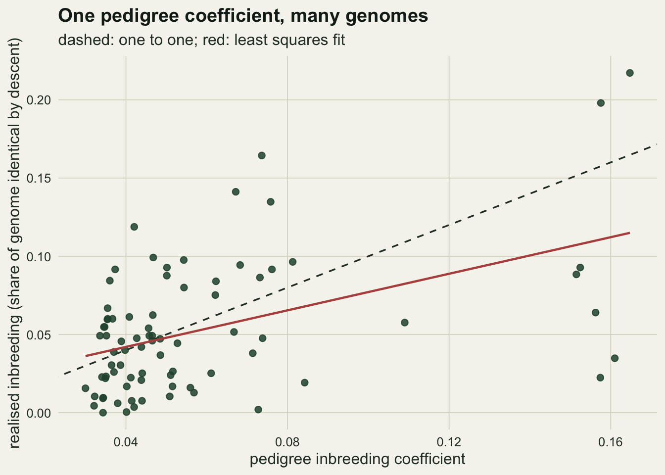
Three measures against the truth
The grid is three SNP densities and four minimum run lengths, on 8 replicate genomes, each with its own pedigree. Three measures are scored against realised inbreeding: the pedigree coefficient, the share of homozygous SNPs, and the share of the genome inside a called run. The densities and thresholds were fixed before the simulation ran and were not revised afterwards. Each density inside a replicate is an independent genome dropped on the same pedigree, which is why the realised mean differs a little between density rows.
set.seed(19840716)
grid_rows <- list(); grid_ind <- list(); kk <- 0
for (rp in seq_len(n_rep)) {
  mate  <- make_ped(n_ind, n_gen)
  f_ped <- ped_f(mate, n_ind, n_gen)
  for (dd in dens_set) {
    pop  <- make_pop(dd, mate)
    fhom <- rowMeans(pop$hom)
    fexc <- f_excess(pop)
    kk   <- kk + 1
    rws  <- data.frame(rep = rp, dens = dd, caller = "strict",
      measure = "pedigree F", min_cm = NA_real_,
      cor = cor(f_ped, pop$f_real), mean = mean(f_ped), false = NA_real_)
    rws  <- rbind(rws, data.frame(rep = rp, dens = dd, caller = "strict",
      measure = "SNP homozygosity", min_cm = NA_real_,
      cor = cor(fhom, pop$f_real), mean = mean(fexc), false = NA_real_))
    roh5 <- NULL
    for (mm in min_set) for (mh in 0:1) {
      rr <- roh_scan(pop, mm, mh)
      rws <- rbind(rws, data.frame(rep = rp, dens = dd,
        caller = c("strict", "one heterozygote allowed")[mh + 1],
        measure = "F_ROH", min_cm = mm,
        cor = safe_cor(rr[, "froh"], pop$f_real), mean = mean(rr[, "froh"]),
        false = mean(rr[, "false"], na.rm = TRUE)))
      if (mm == 5 && mh == 0) roh5 <- rr[, "froh"]
    }
    grid_rows[[kk]] <- rws
    grid_ind[[kk]]  <- data.frame(rep = rp, dens = dd, f_real = pop$f_real,
      f_ped = f_ped, f_exc = fexc, f_roh5 = roh5)
  }
}
grid_tab <- do.call(rbind, grid_rows)
grid_per <- do.call(rbind, grid_ind)

pick <- function(meas, dd, mm = NA, what = "cor", cal = "strict") {
  sel <- grid_tab$measure == meas & grid_tab$dens == dd & grid_tab$caller == cal &
    (if (is.na(mm)) is.na(grid_tab$min_cm) else
       !is.na(grid_tab$min_cm) & grid_tab$min_cm == mm)
  grid_tab[[what]][sel]
}
cell_slope <- vapply(split(grid_per, list(grid_per$rep, grid_per$dens)),
                     function(d) coef(lm(d$f_real ~ d$f_ped))[2], 0)
cell_gap   <- vapply(split(grid_per, list(grid_per$rep, grid_per$dens)),
                     function(d) mean(d$f_real) - mean(d$f_ped), 0)
cell_rep   <- vapply(split(grid_per, list(grid_per$rep, grid_per$dens)),
                     function(d) d$rep[1], 0)
rep_slope <- tapply(cell_slope, cell_rep, mean)
rep_gap   <- tapply(cell_gap, cell_rep, mean)
slope_m   <- mean(rep_slope); slope_sem <- sd(rep_slope) / sqrt(n_rep)
slope_sd_cell <- sd(cell_slope); n_cell <- length(cell_slope)
gap_m     <- mean(rep_gap);   gap_sem   <- sd(rep_gap) / sqrt(n_rep)

ped_cell    <- grid_tab[grid_tab$measure == "pedigree F", ]
ped_cor_all <- tapply(ped_cell$cor, ped_cell$rep, mean)
n_ped_cell  <- nrow(ped_cell)
roh_cor_5_5 <- pick("F_ROH", 5, 5)
n_ped_worse <- sum(ped_cor_all < roh_cor_5_5)
real_mean_d <- tapply(grid_per$f_real, grid_per$dens, mean)
mcse_cor    <- sd(ped_cor_all) / sqrt(n_rep)
The pedigree earns its reputation on the average and loses it on the animal, and both halves are visible in the same eight replicates. Averaged over them, realised inbreeding exceeds the pedigree coefficient by +0.0003 with a standard error of 0.0007, so the pedigree mean is the right number for the annual report. The within-herd regression of realised on pedigree inbreeding has a mean slope of 1.01 with a standard error of 0.05, which covers the value of one that theory requires. Single herds land a long way from it in both directions: across the 24 herd and panel combinations in the grid the fitted slope has a standard deviation of 0.32, which is why the 0.58 of the herd in the first figure is not evidence that a pedigree is biased.
Across the 8 replicates the pedigree coefficient correlates with realised inbreeding at a mean of 0.55, ranging from 0.33 to 0.68 with a standard error on the mean of 0.04. The pedigree coefficient does not depend on the marker panel, so each replicate figure averages the three density cells of that replicate, 24 cells of the same quantity in all. A five centimorgan minimum on a five SNP per centimorgan panel correlates at a mean of 0.983, range 0.970 to 0.992. The run-based coefficient beats the pedigree in 8 of 8 genomes, which is the ranking Keller and colleagues reported and Kardos and colleagues argued for. The replicate spread of the pedigree correlation is the wide one: a single simulated population can land anywhere between a poor and a fair proxy, and a post that ran one replicate could have reported either. That correlation is also specific to this genome rather than to pedigrees in general, and the last section measures how far it moves with the total map length.
hom_cor  <- vapply(dens_set, function(dd) mean(pick("SNP homozygosity", dd)), 0)
roh_best <- vapply(dens_set, function(dd) max(vapply(min_set,
  function(mm) mean(pick("F_ROH", dd, mm)), 0)), 0)
roh_best_cm <- vapply(dens_set, function(dd) min_set[which.max(vapply(min_set,
  function(mm) mean(pick("F_ROH", dd, mm)), 0))], 0)
hom_gap  <- roh_best - hom_cor
roh_1_1  <- mean(pick("F_ROH", 1, 1))
roh_1_10 <- mean(pick("F_ROH", 1, 10))
roh_20_1 <- mean(pick("F_ROH", 20, 1))
lev_20_1 <- mean(pick("F_ROH", 20, 1, "mean"))
lev_5_5  <- mean(pick("F_ROH", 5, 5, "mean"))
lev_5_10 <- mean(pick("F_ROH", 5, 10, "mean"))
bias_5_5 <- lev_5_5 / real_mean_d[["5"]] - 1
bias_20_1 <- lev_20_1 / real_mean_d[["20"]] - 1
exc_mean <- vapply(dens_set, function(dd) mean(pick("SNP homozygosity", dd, what = "mean")), 0)
The homozygosity measure appears in two forms below. Correlations use the raw share of homozygous SNPs; every level and every regression slope uses the excess-homozygosity coefficient, observed minus expected homozygosity over the number of markers minus expected, with the expectation taken from the founder allele frequencies. The two are an affine transform of each other, so the correlation is the same for both while the level is not.
The plain share of homozygous SNPs does better than its reputation. It correlates with realised inbreeding at 0.64 at one SNP per centimorgan, 0.84 at five and 0.96 at twenty. At the densest panel the best run caller reaches 0.999, 0.040 above the homozygosity share, and for a programme that only wants to rank its animals that difference is not worth an argument. Calling runs earns its keep at intermediate density, where the gap is 0.14, and it is at the sparse panel that everything collapses together.
Correlation and level are separate failures, and the sparse and dense ends fail differently. At twenty SNPs per centimorgan with a one centimorgan minimum the correlation is 0.993, as good as any cell in the grid, while the mean called coefficient is 0.075 against a realised mean of 0.057, an overstatement of 33 per cent. Chance runs at a lenient threshold add an almost constant amount to every animal, which leaves the ranking alone and moves the number that goes in the report. At five SNPs per centimorgan with a five centimorgan minimum the mean is 0.0591 for a realised 0.0549, 8 per cent high.
surf <- aggregate(cbind(cor, mean) ~ dens + min_cm,
                  grid_tab[grid_tab$measure == "F_ROH" &
                           grid_tab$caller == "strict", ],
                  function(x) c(m = mean(x), lo = min(x), hi = max(x)))
surf_df <- data.frame(dens = factor(surf$dens, levels = dens_set,
                                    labels = paste(dens_set, "per cM")),
                      min_cm = surf$min_cm,
                      cor = surf$cor[, "m"], cor_lo = surf$cor[, "lo"],
                      cor_hi = surf$cor[, "hi"], lev = surf$mean[, "m"],
                      lev_lo = surf$mean[, "lo"], lev_hi = surf$mean[, "hi"])
dens_col <- c(te_rust, te_gold, te_forest)

p_cor <- ggplot(surf_df, aes(min_cm, cor, colour = dens)) +
  geom_hline(yintercept = mean(ped_cor_all), linetype = "dashed",
             colour = te_body, linewidth = 0.5) +
  geom_hline(yintercept = hom_cor[3], linetype = "dotted",
             colour = te_body, linewidth = 0.5) +
  geom_line(linewidth = 0.9) +
  geom_errorbar(aes(ymin = cor_lo, ymax = cor_hi), width = 0.06, linewidth = 0.5) +
  geom_point(size = 2) +
  scale_colour_manual(values = dens_col, name = "SNPs") +
  scale_x_log10(breaks = min_set) +
  labs(x = "minimum run length (cM)", y = "correlation with realised inbreeding",
       title = "Agreement", subtitle = "dashed pedigree, dotted F_hom") +
  theme_datasheet()

p_lev <- ggplot(surf_df, aes(min_cm, lev, colour = dens)) +
  geom_hline(yintercept = mean(grid_per$f_real), linetype = "dashed",
             colour = te_body, linewidth = 0.5) +
  geom_line(linewidth = 0.9) +
  geom_errorbar(aes(ymin = lev_lo, ymax = lev_hi), width = 0.06, linewidth = 0.5) +
  geom_point(size = 2) +
  scale_colour_manual(values = dens_col, name = "SNPs") +
  scale_x_log10(breaks = min_set) + scale_y_log10() +
  labs(x = "minimum run length (cM)", y = "mean called coefficient",
       title = "Level", subtitle = "dashed: the realised mean") +
  theme_datasheet()

p_cor + p_lev + plot_layout(guides = "collect") +
  plot_annotation(theme = theme_datasheet()) &
  theme(legend.position = "bottom")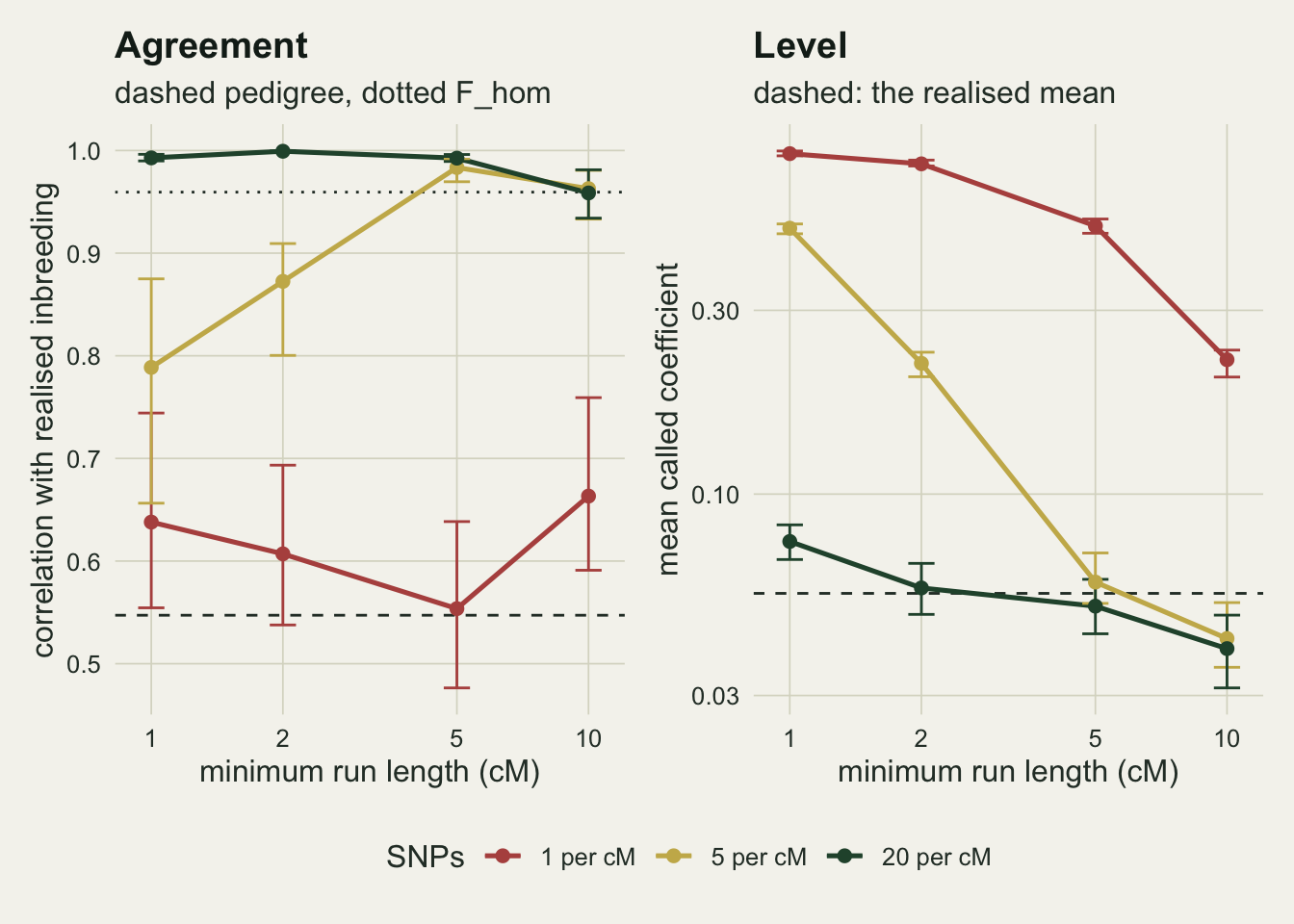
Most called runs are not identical by descent
The share of called run length that is genuinely identical by descent is the quantity a run caller never reports and every reader assumes. It can be computed here because the founder labels are known, and it is the harshest number in the post.
false_get <- function(dd, mm, cal = "strict") mean(pick("F_ROH", dd, mm, "false", cal))
false_tab <- outer(dens_set, min_set, Vectorize(false_get))
dimnames(false_tab) <- list(dens_set, min_set)
false_1_min <- min(false_tab["1", ]); false_1_max <- max(false_tab["1", ])
false_5_5   <- false_tab["5", "5"]; false_5_10 <- false_tab["5", "10"]
false_20_1  <- false_tab["20", "1"]; false_20_5 <- false_tab["20", "5"]
share_1     <- range(vapply(min_set, function(mm) mean(pick("F_ROH", 1, mm, "mean")), 0))

chance_run <- function(dd, mm) chance_hom^(dd * mm)
cr_1_5   <- chance_run(1, 5);  cr_5_5  <- chance_run(5, 5)
cr_20_5  <- chance_run(20, 5); cr_1_10 <- chance_run(1, 10)
cr_5_10  <- chance_run(5, 10)
At one SNP per centimorgan the caller returns between 22 and 77 per cent of the genome as runs, depending on the threshold, and between 82 and 93 per cent of that length is not identical by descent. Raising the minimum run length does not rescue a sparse panel. It only trades one failure for another: the ten centimorgan minimum on that panel still has 82 per cent of its called length false, and by then it is calling only 22 per cent of the genome.
The closed form says why, in one line and with no simulation. A stretch of positions that are not identical by descent is homozygous throughout with probability equal to the chance homozygosity raised to the number of markers in the stretch, because founder alleles here are independent across positions. A five centimorgan window holds 5 markers at one SNP per centimorgan, so it passes by chance with probability 0.237, which is one window in 4.2; the same window holds 25 markers at five SNPs per centimorgan, and the odds fall to one in 1336; at twenty SNPs per centimorgan the window holds 100 markers and the probability is 3.1e-13, which is not a number anyone needs to think about. The minimum run length in centimorgans is not the control variable. The number of markers inside it is.
het_get <- function(dd, mm, what) mean(pick("F_ROH", dd, mm, what,
                                            "one heterozygote allowed"))
het_5_5   <- het_get(5, 5, "false");  het_5_5_lev <- het_get(5, 5, "mean")
het_5_10  <- het_get(5, 10, "false"); het_20_5   <- het_get(20, 5, "false")
het_5_5_c <- het_get(5, 5, "cor")
het_ratio <- het_5_5 / false_5_5
The strict caller is not what PLINK does. Its default scan allows one heterozygous site per window, so that a single genotyping error does not split a genuine run in two, and the question is whether that leniency moves the surface. Allowing one heterozygote anywhere inside a run raises the false share at five SNPs per centimorgan and a five centimorgan minimum from 0.23 to 0.54, a factor of 2.3, and the mean called coefficient from 0.059 to 0.095. The correlation gives up little, from 0.983 to 0.924. At twenty SNPs per centimorgan with the same minimum the false share is 0.054 against 0.024 strict, so the leniency costs little once the panel is dense. This is a harsher rule than PLINK’s, which spends its one heterozygote per window rather than per run and so tolerates more of them in a long run; the direction is the point, and the direction is that leniency is paid for in false length, not in ranking.
false_df <- aggregate(false ~ dens + min_cm + caller,
                      grid_tab[grid_tab$measure == "F_ROH", ], mean)
false_df$dens <- factor(false_df$dens, levels = dens_set,
                        labels = paste(dens_set, "SNP per cM"))
false_df$caller <- factor(false_df$caller,
                          levels = c("strict", "one heterozygote allowed"))

ggplot(false_df, aes(min_cm, false, colour = dens)) +
  geom_line(linewidth = 0.9) +
  geom_point(size = 2) +
  facet_wrap(~ caller) +
  scale_colour_manual(values = dens_col, name = NULL) +
  scale_x_log10(breaks = min_set) +
  scale_y_continuous(limits = c(0, 1)) +
  labs(x = "minimum run length (cM)",
       y = "share of called run length not identical by descent",
       title = "What the caller calls that is not there",
       subtitle = "eight replicate genomes, means") +
  theme_datasheet() +
  theme(legend.position = "bottom",
        strip.text = element_text(colour = te_ink, face = "bold"))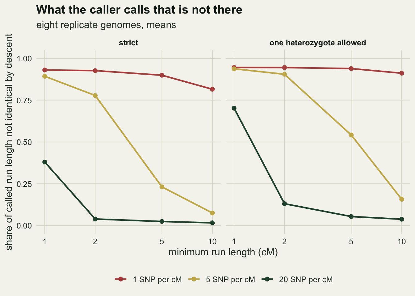
What each measure does to an inbreeding depression slope
Ranking animals is one use for these coefficients. Estimating inbreeding depression is the other, and the two uses do not reward the same measure. A trait is generated with a slope on realised inbreeding, and the slope is then recovered by regressing the trait on each measure in turn.
set.seed(5510)
b_true  <- 3      # decline in the trait per unit of realised inbreeding
sd_resid <- 0.15  # residual standard deviation of the trait
n_fit   <- 100    # trait data sets per genome

fit_one_cell <- function(dsub) {
  est <- replicate(n_fit, {
    yy <- 1 - b_true * dsub$f_real + rnorm(nrow(dsub), 0, sd_resid)
    c(real = -coef(lm(yy ~ dsub$f_real))[2], ped = -coef(lm(yy ~ dsub$f_ped))[2],
      hom  = -coef(lm(yy ~ dsub$f_exc))[2], roh = -coef(lm(yy ~ dsub$f_roh5))[2],
      t_ped = -summary(lm(yy ~ dsub$f_ped))$coefficients[2, 3],
      t_roh = -summary(lm(yy ~ dsub$f_roh5))$coefficients[2, 3],
      t_hom = -summary(lm(yy ~ dsub$f_exc))$coefficients[2, 3])
  })
  data.frame(rep = dsub$rep[1], dens = dsub$dens[1], t(rowMeans(est)))
}
fit_tab <- do.call(rbind, lapply(split(grid_per, list(grid_per$rep, grid_per$dens)),
                                 fit_one_cell))
names(fit_tab)[3:9] <- c("real", "ped", "hom", "roh", "t_ped", "t_roh", "t_hom")

fit_sum <- aggregate(cbind(real, ped, hom, roh, t_ped, t_roh, t_hom) ~ dens,
                     fit_tab, function(x) c(m = mean(x), se = sd(x) / sqrt(n_rep)))
grab <- function(col, dd, what = "m") fit_sum[[col]][fit_sum$dens == dd, what]
ped_by_rep  <- tapply(fit_tab$ped, fit_tab$rep, mean)
ped_slope_m <- mean(ped_by_rep); ped_slope_se <- sd(ped_by_rep) / sqrt(n_rep)
ped_z       <- (ped_slope_m - b_true) / ped_slope_se
The slope on realised inbreeding itself comes back at 3.00 against a generating value of 3.0, which says the machinery works. The pedigree coefficient recovers 3.04 averaged over genomes, with a standard error across genomes of 0.15, 0.3 standard errors from the generating value. The pedigree coefficient does not depend on the marker panel, so the three points on its row in the figure below are three redraws of the genome and the trait on the same eight pedigrees rather than a density effect. Their spread measures how precise a pedigree slope is under a fixed set of pedigrees; it does not include the variation from drawing a different pedigree. That imprecision has a name: it is the Berkson property of a pedigree, realised inbreeding scatters around the pedigree coefficient rather than the other way round, so the pedigree gives an unbiased slope and pays for it in precision.
roh_slope_5 <- grab("roh", 5); roh_se_5 <- grab("roh", 5, "se")
roh_slope_1 <- grab("roh", 1); hom_slope_20 <- grab("hom", 20)
hom_slope_1 <- grab("hom", 1); roh_slope_20 <- grab("roh", 20)
att_roh_1   <- 1 - roh_slope_1 / b_true
att_hom_20  <- 1 - hom_slope_20 / b_true
t_ratio_5   <- grab("t_roh", 5) / grab("t_ped", 5)
t_ratio_20  <- grab("t_roh", 20) / grab("t_ped", 20)
The marker measures go the other way. They are realised inbreeding plus measurement error, which is the classical case, so their slopes attenuate towards zero. At five SNPs per centimorgan the five centimorgan caller returns 2.79 with a standard error of 0.03; at twenty SNPs per centimorgan it returns 3.00; at one SNP per centimorgan it returns 1.51, 50 per cent short. The homozygosity share attenuates at every density, by 8 per cent even on the densest panel, because it counts chance homozygosity as inbreeding at every position. This is the attenuation Kardos and colleagues (2015) warn about, and it runs in the opposite direction to the pedigree’s error.
The practical consequence is in the test statistic rather than the estimate. The mean t statistic for the run-based measure is 2.6 times the pedigree’s at five SNPs per centimorgan and 2.1 times it at twenty. A programme that reports an attenuated slope with a small standard error has a different problem from one that reports an unbiased slope it cannot distinguish from zero, and only the second problem is solved by more animals.
fit_long <- do.call(rbind, lapply(c("real", "ped", "hom", "roh"), function(cl)
  data.frame(measure = cl, dens = fit_sum$dens, est = fit_sum[[cl]][, "m"],
             se = fit_sum[[cl]][, "se"])))
fit_long$measure <- factor(fit_long$measure, levels = c("roh", "hom", "ped", "real"),
  labels = c("F_ROH, 5 cM", "SNP homozygosity", "pedigree F", "realised inbreeding"))
fit_long$dens <- factor(fit_long$dens, levels = dens_set,
                        labels = paste(dens_set, "SNP per cM"))

ggplot(fit_long, aes(est, measure, colour = dens)) +
  geom_vline(xintercept = b_true, linetype = "dashed",
             colour = te_body, linewidth = 0.6) +
  geom_errorbar(aes(xmin = est - se, xmax = est + se), orientation = "y",
                width = 0.25, linewidth = 0.5,
                position = position_dodge(width = 0.55)) +
  geom_point(size = 2.4, position = position_dodge(width = 0.55)) +
  scale_colour_manual(values = dens_col, name = NULL) +
  labs(x = "recovered slope", y = NULL,
       title = "Two kinds of error, two directions",
       subtitle = "dashed: the generating slope, fixed before the run") +
  theme_datasheet() + theme(legend.position = "bottom")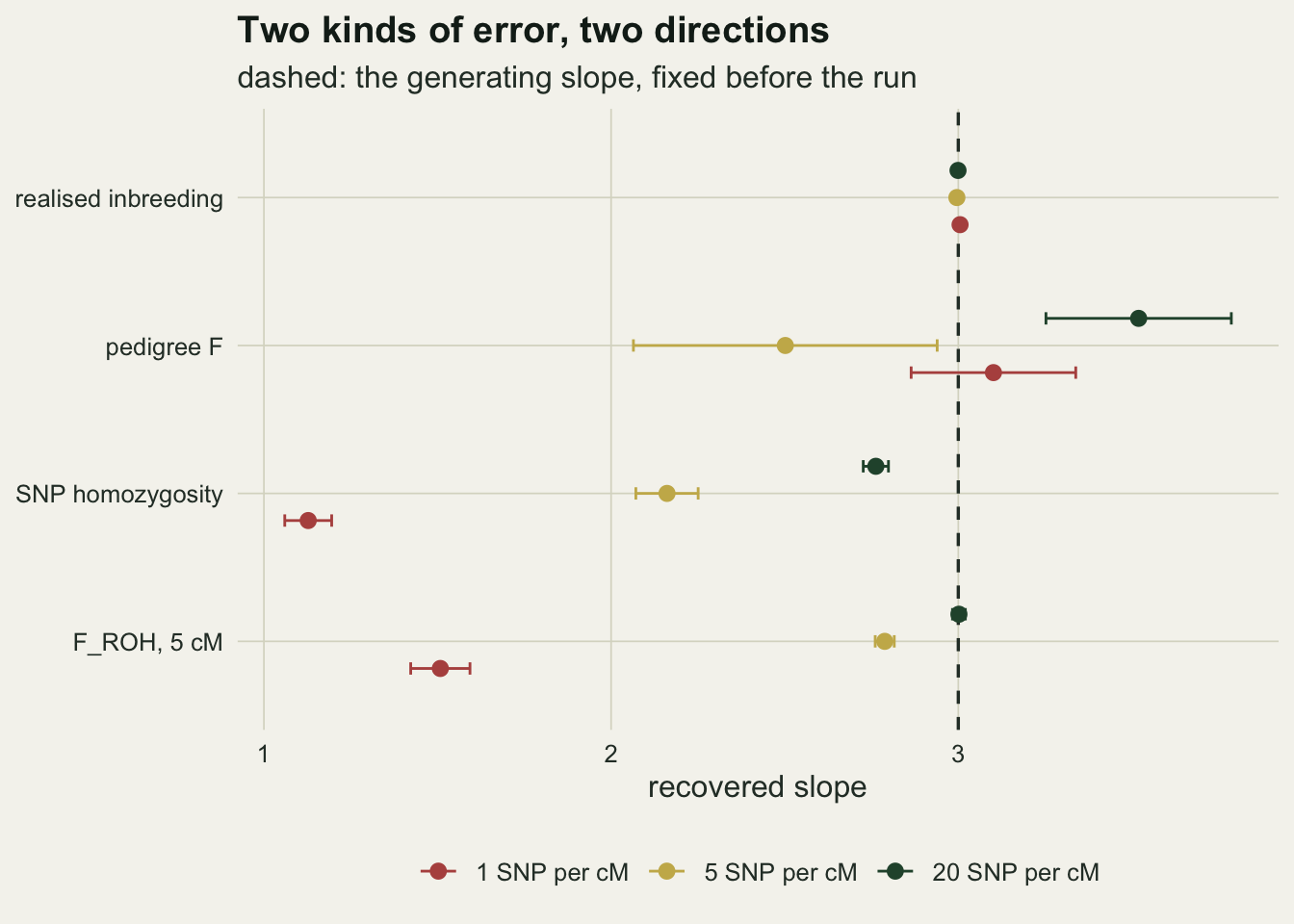
Three things the simulation was set up to get wrong
Three design choices in the main grid work in the run caller’s favour, and each can be measured rather than confessed. The founders carry no linkage disequilibrium, so chance homozygosity is independent from marker to marker and chance runs are as short as they can be. The genome is five long chromosomes rather than twenty short ones of the same total length, so the identical material sits in fewer and longer pieces. And the whole map is five morgans, which leaves more Mendelian sampling variance for the pedigree to miss than a real genome would.
set.seed(31337)
ld_set  <- c(0, 5, 20)
n_anc_ld <- 8
ld_rep  <- 3
ld_rows <- list(); kk <- 0
for (rp in seq_len(ld_rep)) {
  mate <- make_ped(n_ind, n_gen)
  for (lc in ld_set) {
    pop <- make_pop(5, mate, ld_cm = lc, n_anc = n_anc_ld)
    rr  <- roh_scan(pop, 5)
    kk  <- kk + 1
    ld_rows[[kk]] <- data.frame(rep = rp, ld = lc,
      chance = mean(pop$hom[!pop$ibd]), froh = mean(rr[, "froh"]),
      false = mean(rr[, "false"], na.rm = TRUE),
      only  = mean(rr[, "only"], na.rm = TRUE),
      anc_bg = mean(pop$anc_ibd[!pop$ibd]), f_anc = mean(pop$f_anc),
      cor = safe_cor(rr[, "froh"], pop$f_real),
      cor_anc = safe_cor(rr[, "froh"], pop$f_anc))
  }
}
ld_tab <- do.call(rbind, ld_rows)
ld_sum <- aggregate(cbind(chance, froh, false, only, anc_bg, f_anc, cor, cor_anc) ~ ld,
                    ld_tab, mean)
ld_get <- function(lc, cl) ld_sum[[cl]][ld_sum$ld == lc]
old_of_false <- 1 - ld_get(20, "only") / ld_get(20, "false")
anc_enrich   <- ld_get(20, "anc_bg")

arch_rep <- 6
arch_rows <- list(); kk <- 0
for (rp in seq_len(arch_rep)) {
  mate  <- make_ped(n_ind, n_gen)
  f_ped <- ped_f(mate, n_ind, n_gen)
  for (ar in 1:2) {
    pop <- if (ar == 1) make_pop(5, mate, n_chr = 5, chr_len = 100) else
                        make_pop(5, mate, n_chr = 20, chr_len = 25)
    kk  <- kk + 1
    arch_rows[[kk]] <- data.frame(rep = rp,
      arch = c("5 x 100 cM", "20 x 25 cM")[ar],
      cor_ped = cor(f_ped, pop$f_real), dev_sd = sd(pop$f_real - f_ped))
  }
}
arch_tab <- do.call(rbind, arch_rows)
arch_get <- function(ar, cl) mean(arch_tab[[cl]][arch_tab$arch == ar])
dev_drop  <- arch_tab$dev_sd[arch_tab$arch == "5 x 100 cM"] -
             arch_tab$dev_sd[arch_tab$arch == "20 x 25 cM"]
cor_rise  <- arch_tab$cor_ped[arch_tab$arch == "20 x 25 cM"] -
             arch_tab$cor_ped[arch_tab$arch == "5 x 100 cM"]
n_dev_dn  <- sum(dev_drop > 0); n_cor_up <- sum(cor_rise > 0)

len_rep <- 6
len_set <- c(5, 20)       # chromosomes of 100 cM, so 5 and 20 morgans of map
len_rows <- list(); kk <- 0
for (rp in seq_len(len_rep)) {
  mate  <- make_ped(n_ind, n_gen)
  f_ped <- ped_f(mate, n_ind, n_gen)
  for (nc in len_set) {
    pop <- make_pop(5, mate, n_chr = nc, chr_len = 100)
    rr  <- roh_scan(pop, 5)
    kk  <- kk + 1
    len_rows[[kk]] <- data.frame(rep = rp, morgan = nc,
      cor_ped = cor(f_ped, pop$f_real), dev_sd = sd(pop$f_real - f_ped),
      cor_roh = safe_cor(rr[, "froh"], pop$f_real))
  }
}
len_tab <- do.call(rbind, len_rows)
len_get <- function(mg, cl) mean(len_tab[[cl]][len_tab$morgan == mg])
n_len_up <- sum(len_tab$cor_ped[len_tab$morgan == 20] >
                len_tab$cor_ped[len_tab$morgan == 5])
Founder linkage disequilibrium was added by building each founder haplotype as a mosaic of 8 ancestral haplotypes, with a switch every 5 or 20 centimorgans on average. Chance homozygosity rises only a little, from 0.752 to 0.783, because the marginal allele frequencies are unchanged. Scored against the founder labels the false share does not rise a little. At five SNPs per centimorgan and a five centimorgan minimum it goes from 0.26 with independent founders to 0.68 at a five centimorgan mosaic and 0.73 at a twenty centimorgan mosaic, and the correlation with realised inbreeding falls from 0.98 to 0.70.
That reads like a caller that has started inventing runs, and it is not one. Founders built from 8 ancestral haplotypes are related to each other, so the founder labels stop being the whole truth about identity by descent and the caller is being marked against a base population that has moved underneath it. Carrying the ancestral haplotype index next to the founder label costs nothing and separates the two. Of the called length that the founder labels score false at the twenty centimorgan mosaic, 78 per cent is positions where both of the animal’s haplotypes copy the same ancestral haplotype, against a background of 0.13 between haplotypes that are not identical by descent from the founders. That is identity by descent older than the pedigree’s base population, and the caller is finding it rather than making it up.
Credit it, and the arm says the opposite of what it first appeared to say. The share of called length that is identical by descent from neither the founders nor an ancestral haplotype is 0.16 at the twenty centimorgan mosaic and 0.22 at the five centimorgan one, against 0.26 with independent founders: lower, not higher. Scoring the correlation against ancestral identity, which is what the markers are actually reading, gives 0.96 at the twenty centimorgan mosaic instead of 0.70. So this arm does not show that the false shares of the main grid are a lower bound. It shows that a false share is a statement about a chosen base population, and that moving the base from the founders of this pedigree to a set of 8 ancestral haplotypes turns the same called length from mostly false into mostly true. What founder haplotype structure costs a real caller in genuine chance runs is not measured here: the mosaic switches at a constant rate, which is not how real haplotype lengths are distributed, and separating old descent from chance needs a coalescent burn-in rather than a mosaic.
Hill and Weir (2011) write the variance of realised relationship around its pedigree expectation in terms of the total map length, and total map length is what the main grid never varies. The length arm fixes that. It holds the pedigree and the panel density and drops the same breeding history onto five chromosomes of one hundred centimorgans and onto twenty of the same length, four times the map. The standard deviation of the deviation between realised and pedigree inbreeding falls from 0.0394 to 0.0209, and the pedigree correlation rises from 0.57 to 0.80, up in 5 of 6 paired replicates. The prediction holds and it holds on length. The pedigree correlation quoted everywhere else in this post is a number about a five morgan genome, and a real vertebrate map of several thousand centimorgans would make the studbook a better individual proxy than any pedigree number here. The run caller barely notices the change, 0.98 to 0.99, because it reads whatever segments it is given.
Splitting a map of fixed length into more chromosomes does much less. Five chromosomes of one hundred centimorgans against twenty of twenty five, five morgans either way: the deviation standard deviation falls from 0.0429 to 0.0370, down in 6 of 6 paired replicates, and the pedigree correlation rises from 0.52 to 0.60, up in 4 of 6. After ten generations of a closed population the identical segments are already chopped into many pieces by recombination, so drawing more chromosome boundaries through a genome that is already fragmented buys less than adding map does. For a reader deciding whether these numbers transfer to their species, the total map is the quantity to check, not the karyotype.
ld_plot <- data.frame(
  lab = factor(rep(c("none", "5 cM", "20 cM"), 2),
               levels = c("none", "5 cM", "20 cM")),
  base = factor(rep(c("founder labels", "ancestral haplotypes"), each = 3),
                levels = c("founder labels", "ancestral haplotypes")),
  share = c(ld_sum$false, ld_sum$only))

p_ld <- ggplot(ld_plot, aes(lab, share, colour = base, group = base)) +
  geom_line(linewidth = 0.9) +
  geom_point(size = 2.8) +
  scale_colour_manual(values = c(te_rust, te_forest), name = "descent scored against") +
  scale_y_continuous(limits = c(0, 1)) +
  labs(x = "founder haplotype mosaic",
       y = "share of called run length not IBD",
       title = "Founder linkage",
       subtitle = "5 SNP per cM, 5 cM minimum") +
  theme_datasheet()

len_plot <- len_tab
len_plot$arch <- factor(ifelse(len_plot$morgan == 5, "5 x 100 cM", "20 x 100 cM"),
                        levels = c("5 x 100 cM", "20 x 100 cM"))
len_mean <- aggregate(cor_ped ~ arch, len_plot, mean)

p_len <- ggplot(len_plot, aes(arch, cor_ped)) +
  geom_line(aes(group = rep), colour = te_body, alpha = 0.35, linewidth = 0.6) +
  geom_point(colour = te_forest, size = 2.2) +
  geom_point(data = len_mean, shape = 18, size = 4.5, colour = te_ink) +
  labs(x = "total map length", y = "pedigree correlation with realised F",
       title = "Genome length",
       subtitle = "paired; diamonds are means") +
  theme_datasheet()

p_ld + p_len + plot_layout(guides = "collect") +
  plot_annotation(theme = theme_datasheet()) &
  theme(legend.position = "bottom")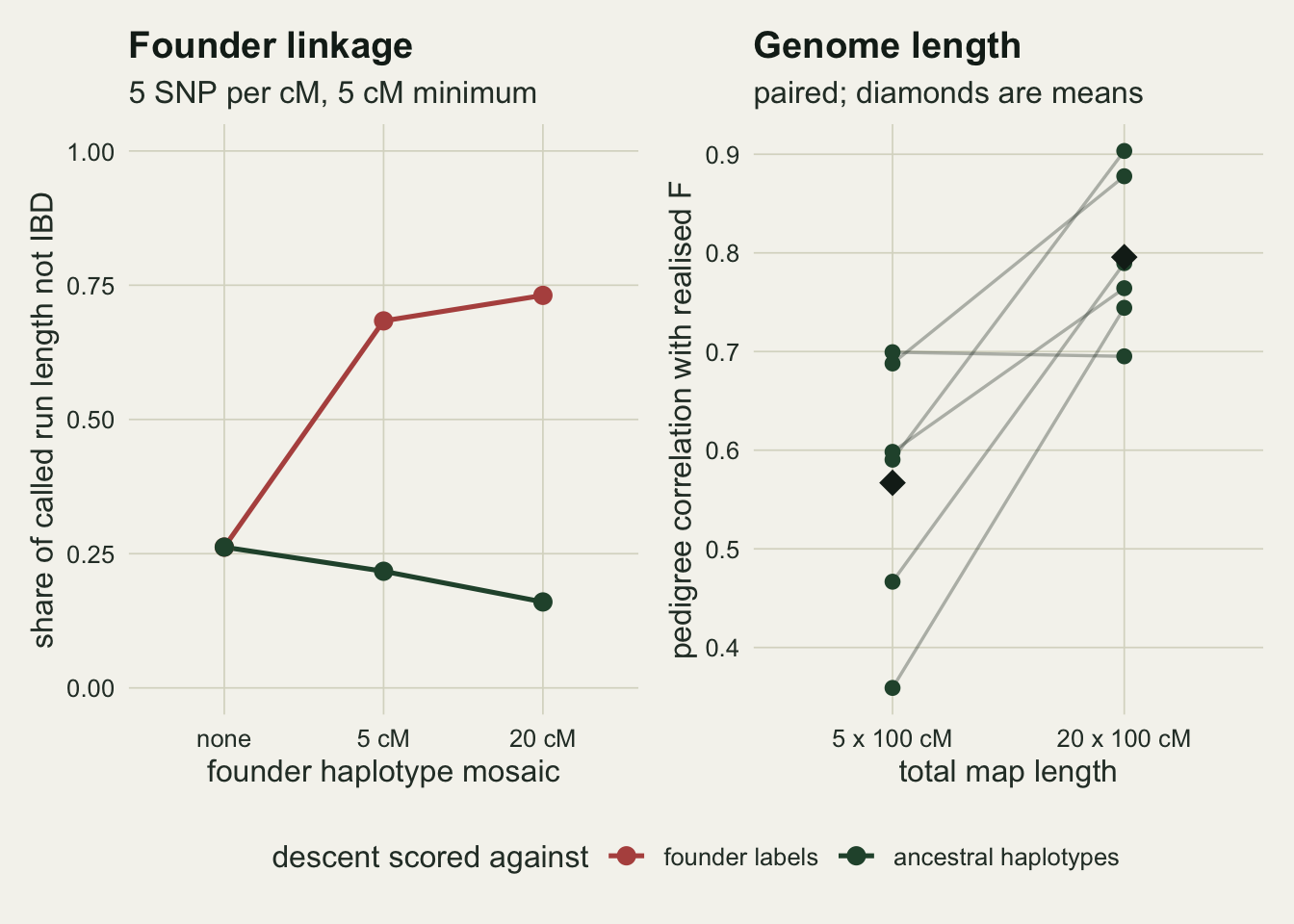
What to report
Report the SNP density of the panel in markers per centimorgan, not in total marker count. A fifty thousand marker panel on a genome of thirty five hundred centimorgans is fourteen markers per centimorgan; the same panel on a thousand centimorgan map is fifty per centimorgan, and the two are different instruments with the same specification sheet. The false-run surface and the run caller’s correlation move with markers per centimorgan and not with the raw count. The pedigree correlation is the exception in the other direction: it does not see the markers at all, and it moves with the total map length.
Report the minimum run length in markers as well as in centimorgans, because that is the quantity the false-run arithmetic uses. At the sparse end of the grid here a five centimorgan minimum is five markers and passes by chance in 24 per cent of non-inherited windows; at five markers per centimorgan the same physical length is twenty five markers and passes in one window in 1336. One line of R, 0.75 raised to the number of markers, tells a reviewer whether a threshold was ever going to work.
Give the mean called coefficient and a ranking statistic separately. They fail independently: the twenty marker per centimorgan panel with a one centimorgan minimum ranks animals at a correlation of 0.993 and overstates the mean by 33 per cent. If the number goes into a management target, the level matters; if it is used to pick pairs, the ranking does.
Do not report a pedigree coefficient as the individual’s inbreeding when a dense panel exists. It is right on average and wrong on the animal: over eight simulated herds the pedigree mean missed the realised mean by 0.0003, while animals sharing a pedigree coefficient differ in realised inbreeding by a factor of several. The pedigree is still the right thing to report for the population mean, for the expected consequence of a proposed pairing, and for any animal without genotypes.
State which measure carried an inbreeding depression slope. An unbiased but imprecise slope from the pedigree and an attenuated but precise slope from a marker measure are different claims, and a paper that does not say which measure it regressed on has not said what its slope estimates.
Honest limits
Founders carry no linkage disequilibrium in the main grid, and the arm that relaxes it turns out to be a statement about the base population rather than about the caller. With founder haplotypes built as mosaics of a small ancestral set, the founder labels score 0.73 of the called length false at the working cell, but 78 per cent of that is descent from a shared ancestral haplotype and the share that is descent from neither base falls to 0.16. So the false shares in the main grid are the right number for the base the pedigree uses, and they are not a lower bound on the false share against a deeper base, because a deeper base makes more of the called length true. What no arm here measures is the extra genuinely chance run length that a realistic distribution of founder haplotype lengths would add; the mosaic switches at a constant rate, and a coalescent burn-in would be the way to get that.
The genome is five morgans, and the length arm says how much of the pedigree’s poor performance is a statement about that choice. Four times the map takes the pedigree correlation from 0.57 to 0.80 while the run caller stays near 0.99. Read every pedigree correlation in this post as belonging to a short genome. The run caller’s advantage over the pedigree is real at any length tested here, but its size is not transferable.
Crossovers are Poisson along each chromosome, with no obligate chiasma and no interference, which is the most permissive meiosis available. A hundred centimorgan chromosome passes through a parent intact whenever its Poisson count comes up zero, which a real bivalent with an obligate chiasma never does, and interference spaces the crossovers that do happen more evenly than uniform positions do. Both make the transmitted share of a parent’s genome less variable in a real meiosis than in this one, so the scatter of realised around pedigree inbreeding here is an upper bound for that reason as well as for the map length.
The genotypes have no errors and no missing calls. Real panels have both, and a single miscalled heterozygote inside a genuine run is exactly what PLINK’s one-heterozygote-per-window default exists to survive. The lenient caller measured here is a harsher rule than PLINK’s, since it spends the allowance on the whole run rather than on a window, so the numbers should be read as the direction of the leniency effect and not as a reproduction of the software’s behaviour.
The founder frequency spectrum is fixed at a beta with both parameters one half. That is a reasonable stand-in for an ascertained SNP panel and it sets the chance homozygosity at 0.75. A panel with more intermediate frequencies has lower chance homozygosity and forgives a sparse marker set more; a panel dominated by rare variants is worse than anything measured here. No result in this post transfers to a different spectrum without rerunning the code with the right one.
The homozygosity measure has a base population problem that the correlation hides. Its excess-homozygosity form needs expected homozygosity, and which allele frequencies supply it decides what the number means. Using the founder frequencies gives a mean of 0.045 at five markers per centimorgan against a realised 0.055; using the current generation’s own frequencies, which is what software does when the base population is not genotyped, sets the base to the inbred present and returns -0.014 in the herd of the first figure. The correlations reported here are unaffected, because correlation does not see a linear rescaling, but every level is.
The population is small, closed and mated at random for ten generations, so realised inbreeding runs around 0.06 and the segments are already well fragmented. A population with recent close matings carries long segments that any caller finds, and one with a deep bottleneck many generations back carries short ones that only a dense panel finds. McQuillan and colleagues (2008) use exactly that relation, run length against age of the ancestral loop, to read demographic history out of the runs, and nothing here separates old from recent inbreeding.
Eight replicate genomes is few. The Monte Carlo standard error on the mean pedigree correlation is 0.04, so differences in that quantity smaller than about 0.08 should not be ranked, and the length and architecture arms are reported as paired counts of replicates rather than as differences for the same reason. The run-based correlations at the working cell are far more stable across replicates than the pedigree correlation is, which is itself part of the result.
The realised inbreeding used as the truth is the share of the genome identical by descent from the founders of this pedigree. Founders are treated as unrelated and non-inbred, which is the same convention the pedigree uses, so both measures share a base population while the marker measures do not. That is a convention, not a fact about any real founder set, and it is the reason the pedigree can be unbiased for the mean here in a way it rarely is in a real studbook. The founder linkage arm is what happens when the convention is broken on purpose, and it is why a false-run share means nothing without the base population it was scored against.
References
Keller MC, Visscher PM, Goddard ME 2011 Genetics 189(1):237-249 (10.1534/genetics.111.130922)
Kardos M, Luikart G, Allendorf FW 2015 Heredity 115(1):63-72 (10.1038/hdy.2015.17)
McQuillan R, Leutenegger AL, Abdel-Rahman R et al. 2008 American Journal of Human Genetics 83(3):359-372 (10.1016/j.ajhg.2008.08.007)
Hill WG, Weir BS 2011 Genetics Research 93(1):47-64 (10.1017/S0016672310000480)
Purcell S, Neale B, Todd-Brown K et al. 2007 American Journal of Human Genetics 81(3):559-575 (10.1086/519795)