Repeating an analysis for every site in R

Fit the same model at every site in R with split, lapply and purrr, and catch the silent faults: sapply changing shape, empty loops and failed sites dropped.

Thirty sites in a monitoring scheme, ten years of counts at each, and a request for the trend at every site. The first version of the script fits the model for site 1, then the block is copied and the 1 becomes a 2. By site 12 one of the copies has a typo in it, and nothing says so. Why copies drift apart, and what it costs, is measured in Turning your code into an R package. This post is about the step before that: writing the analysis once and running it for every site.

Running it is the easy part. R has several ways to repeat a function over groups, and the differences that matter here are not about speed but about what each one does when a site is unusual. That is where the plausible wrong numbers come from: a result that changes shape because one site had a tie, a loop that runs even when there is nothing to loop over, and a summary that quietly leaves out the sites where the model failed. Each of those is shown below on one simulated survey, measured, and then fixed.

Speed is a separate question with its own post, Speeding up your analysis code; here every loop is quick, and the question is only whether its answer is right. If all you need is one number per group, such as a mean, Summarising ecological data by group covers group_by() and summarise().

The short answer

Write a function that does the analysis for one site and returns one row, or one number. Run it on a single site and read the result. Then split the data by site and apply the function to every piece with lapply() or purrr::map(), and bind the rows together. When each site returns one number, use vapply() or purrr::map_dbl() instead of sapply(), because they stop when a site returns something else. Loop over seq_along(x), never 1:length(x). And when a site can fail, keep it in the output as NA with its name, so the failures can be counted and looked at before anything is averaged.

The survey

The data are simulated, so that we know the true trend at every site and can score each answer against it. Each site enters the scheme in 2015 with its own expected count and then changes by its own fixed rate per year. The counts are Poisson around that expectation. In your own data you never see the true_trend column; here it is the answer key.

library(dplyr)
library(purrr)
library(ggplot2)

set.seed(2026)
n_site <- 30
years  <- 2015:2024
sites <- data.frame(
  site       = sprintf("S%02d", seq_len(n_site)),
  region     = rep(c("north", "south"), each = n_site / 2),
  count_2015 = exp(rnorm(n_site, log(10), 0.7)),  # expected count in the first year
  true_trend = rnorm(n_site, -0.03, 0.08)         # change per year, log scale
)
survey <- expand.grid(year = years, site = sites$site, stringsAsFactors = FALSE) |>
  left_join(sites, by = "site") |>
  mutate(count = rpois(n(), count_2015 * exp(true_trend * (year - 2015)))) |>
  select(site, region, year, count)

head(survey, 3)

  site region year count
1  S01  north 2015    13
2  S01  north 2016    14
3  S01  north 2017    11

nrow(survey)

[1] 300

300 rows: 30 sites, 10 years each, one count per visit.

One site first, then every site

The analysis for one site is a linear regression of count on year, and the number we want from it is the slope: the change in individuals per year. Write it as a function of one site’s rows, and make it return a one-row data frame, so that the rows from all sites stack into a table.

site_trend <- function(d) {
  fit <- lm(count ~ year, data = d)
  data.frame(site = d$site[1], n_years = nrow(d), slope = coef(fit)[["year"]])
}
by_site <- split(survey, survey$site)
site_trend(by_site[["S01"]])

  site n_years     slope
1  S01      10 -0.969697

split() turns the table into a list with one data frame per site, named by site. Checking the function on one element of that list, and comparing the answer with what you expect from a plot of that site, is the step that is worth the time. After that, repeating it is one line, and there are three common ways to write that line.

# base R: apply to every piece, then stack the rows
trends <- do.call(rbind, lapply(by_site, site_trend))
# purrr: the same, with a binding function that expects data frames
trends_purrr <- map(by_site, site_trend) |> list_rbind()
# dplyr: fine when the result is one number per site
trends_dplyr <- survey |>
  group_by(site) |>
  summarise(slope = coef(lm(count ~ year))[["year"]])

stopifnot(all.equal(trends$slope, trends_purrr$slope),
          all.equal(trends$slope, trends_dplyr$slope))
head(trends_purrr, 4)

  site n_years      slope
1  S01      10 -0.9696970
2  S02      10 -0.2363636
3  S03      10 -0.9393939
4  S04      10  0.2787879

All three give the same 30 slopes, and the stopifnot() line checks that they do. The slopes run from -2.59 to 3.21 individuals per year. Which of the three to use is mostly taste. The lapply() and map() versions scale to anything the function returns, including a whole model object; the summarise() version is the shortest when one number per site is all you need.

sapply() decides the shape for you

A second question for the same data: in which year was each site at its peak? The obvious function returns the year, or years, with the highest count.

peak_year <- function(d) d$year[d$count == max(d$count)]
class(sapply(by_site[1:5], peak_year))

[1] "integer"

class(sapply(by_site, function(d) range(d$count)))

[1] "matrix" "array" 

peak <- sapply(by_site, peak_year)
class(peak)

[1] "list"

lengths(peak)[lengths(peak) > 1]

S15 S17 
  2   2 

sapply() looks at what came back and chooses a shape. For the first five sites every answer had length one, and the result was a plain integer vector. For a function that returns two numbers per site, such as range(), it builds a matrix. For all 30 sites the result is a list, because 2 sites (S15 and S17) had the same highest count in two years. The same line of code gives a different kind of object depending on the data it meets, and the code after it was written for one of those kinds.

Sometimes the next line fails, which is the good outcome. Sometimes it does not:

length(unlist(peak))

[1] 32

mean(unlist(peak))

[1] 2018.812

unlist() flattens the list into 32 years for 30 sites, and the mean runs without a message. The tied sites count twice, and nothing in the output says so. This is why Wickham (2019, section 9.2.1) advises keeping sapply() out of scripts that run unattended.

vapply() and map_dbl() are told in advance what each result must look like, and they refuse anything else:

err_v <- tryCatch(vapply(by_site, peak_year, numeric(1)), error = function(e) e)
conditionMessage(err_v)

[1] "values must be length 1,\n but FUN(X[[15]]) result is length 2"

err <- tryCatch(map_dbl(by_site, peak_year), error = function(e) e)
err$name

[1] "S15"

conditionMessage(err$parent)

[1] "Result must be length 1, not 2."

Both stop at the first tied site, and both say which one it was: vapply() by its position in the list, map_dbl() by position and by name (S15). The error is not the problem to solve; it is the message that your function has no rule for ties. Give it one, for example the first year the peak was reached, and the strict version runs:

first_peak <- function(d) d$year[which.max(d$count)]
peak_fixed <- vapply(by_site, first_peak, numeric(1))
length(peak_fixed)

[1] 30

Now there are 30 years for 30 sites, and the next time the data change shape, the line stops instead of guessing.

A loop that runs over nothing

for loops are fine in R, and for a first script they are often clearer than lapply(). The trap is in how the loop counts. Suppose the analysis is restricted to one region, and the region is typed with a capital letter that the data do not use:

north <- unique(survey$site[survey$region == "North"])
length(north)

[1] 0

1:length(north)

[1] 1 0

totals <- numeric(0)
for (i in 1:length(north)) {
  totals[i] <- sum(survey$count[survey$site == north[i]], na.rm = TRUE)
}
totals

[1] 0

The filter matched no site, so there is nothing to total, and yet totals has 1 element, a total of 0 individuals. 1:length(north) is 1:0, which counts down to the vector c(1, 0), so the loop ran twice. On the first pass north[1] is NA, every comparison with it is NA, and sum(..., na.rm = TRUE) of nothing but NA is zero. On the second pass it assigned to position zero, which R ignores. The result looks like a site where nothing was counted.

totals <- numeric(0)
for (i in seq_along(north)) {
  totals[i] <- sum(survey$count[survey$site == north[i]], na.rm = TRUE)
}
length(totals)

[1] 0

seq_along(north) is empty when north is empty, so the loop body never runs and the result has length 0; Wickham (2019, section 5.3.1) lists 1:length(x) among the common loop pitfalls for this reason. Better still, say what you expect before the loop starts: stopifnot(length(north) > 0) turns the typo into an error on the line where it happened. Why a check at the top is worth its lines is the subject of Debugging and defensive R code.

When one site fails

The trend in individuals per year is hard to compare between a site with 5 individuals and one with 50. A common next step is to fit the log of the count, so that the slope becomes a proportional change, and to report it as per cent change per year.

pct_trend <- function(d) {
  fit <- lm(log(count) ~ year, data = d)
  100 * (exp(coef(fit)[["year"]]) - 1)
}
pct_trend(by_site[["S01"]])

[1] -13.05201

It works on site 1. It does not work on every site, because the log of a zero count is minus infinity and lm() stops with an error. In a loop, the first failing site stops everything:

pct_loop <- setNames(rep(NA_real_, n_site), names(by_site))
err_loop <- tryCatch(
  for (i in seq_along(by_site)) pct_loop[i] <- pct_trend(by_site[[i]]),
  error = function(e) e)
conditionMessage(err_loop)

[1] "NA/NaN/Inf in 'y'"

sum(!is.na(pct_loop))

[1] 5

The loop filled 5 sites and then stopped at S06, the first site with a zero count. lapply() is worse in one respect: it returns nothing at all, so the results for the sites before the failure are gone too. Both at least stop, and you know something went wrong.

The usual next move is to catch the error and carry on. purrr::possibly() wraps a function so that an error returns a value of your choice instead. What that value is decides whether the failed sites stay visible.

pct_dropped <- map(by_site, possibly(pct_trend)) |> list_c()
length(pct_dropped)

[1] 24

names(pct_dropped)

NULL

pct <- map_dbl(by_site, possibly(pct_trend, otherwise = NA_real_))
length(pct)

[1] 30

names(pct)[is.na(pct)]

[1] "S06" "S08" "S13" "S15" "S21" "S23"

The first version uses the default of possibly(), which returns NULL on an error, and list_c() drops the NULL elements, and it never keeps the outer names, so the site names go too. The result is 24 numbers with no names, and nothing tells you that 6 sites are missing, or which. The second version returns NA on an error, and map_dbl() keeps one named value per site: 24 trends and 6 NA values, with the failed sites listed by name. The same holds in base R: tryCatch(pct_trend(d), error = function(e) NA_real_) inside vapply() does the same job.

The failed sites are not a random sample

A named NA does more than keep the count right. It lets you ask what the failed sites have in common, and here the answer matters. A site fails when it has a zero count in at least one year. In a year with an expected count of mu individuals, the chance of a Poisson count of zero is exp(-mu): less than one in ten thousand when mu is 10, 2 per cent when it is 4 and 37 per cent when it is 1. So a site reaches zero when it starts small or when it declines. The simulated survey has the answer key, so we can compare the true trends of the two groups.

scored <- sites |>
  mutate(estimate = unname(pct[site]),
         status = if_else(is.na(estimate), "failed", "fitted"),
         true_pct = 100 * (exp(true_trend) - 1))
scored |> group_by(status) |> summarise(sites = n(), mean_true_pct = mean(true_pct))

# A tibble: 2 × 3
  status sites mean_true_pct
  <chr>  <int>         <dbl>
1 failed     6         -7.62
2 fitted    24         -2.99

truth_all  <- mean(scored$true_pct)
report_fit <- mean(scored$estimate, na.rm = TRUE)
c(true_mean_all_sites = truth_all, reported_mean = report_fit)

true_mean_all_sites       reported_mean 
          -3.917224           -3.444762 

The 6 sites that failed were declining by 7.6 per cent per year on average, against 3.0 per cent for the sites that were fitted. The mean of the reported trends is -3.4 per cent per year; the true mean over all 30 sites is -3.9. 5 of the 6 failed sites were declining. The other one, S06, was increasing but started from an expected count of 1.7 individuals, low enough for a zero in the early years. The summary made the scheme look healthier than it is, because the model failed mostly at sites where the species was declining fast.

Figure 1: True trend of each of the 30 simulated sites, ordered from steepest decline to strongest increase. Sites where the log-count model failed are in red; most of them sit among the steepest declines. The dashed line is the true mean over all sites and the solid line is the mean of the trends that the fitted sites reported.

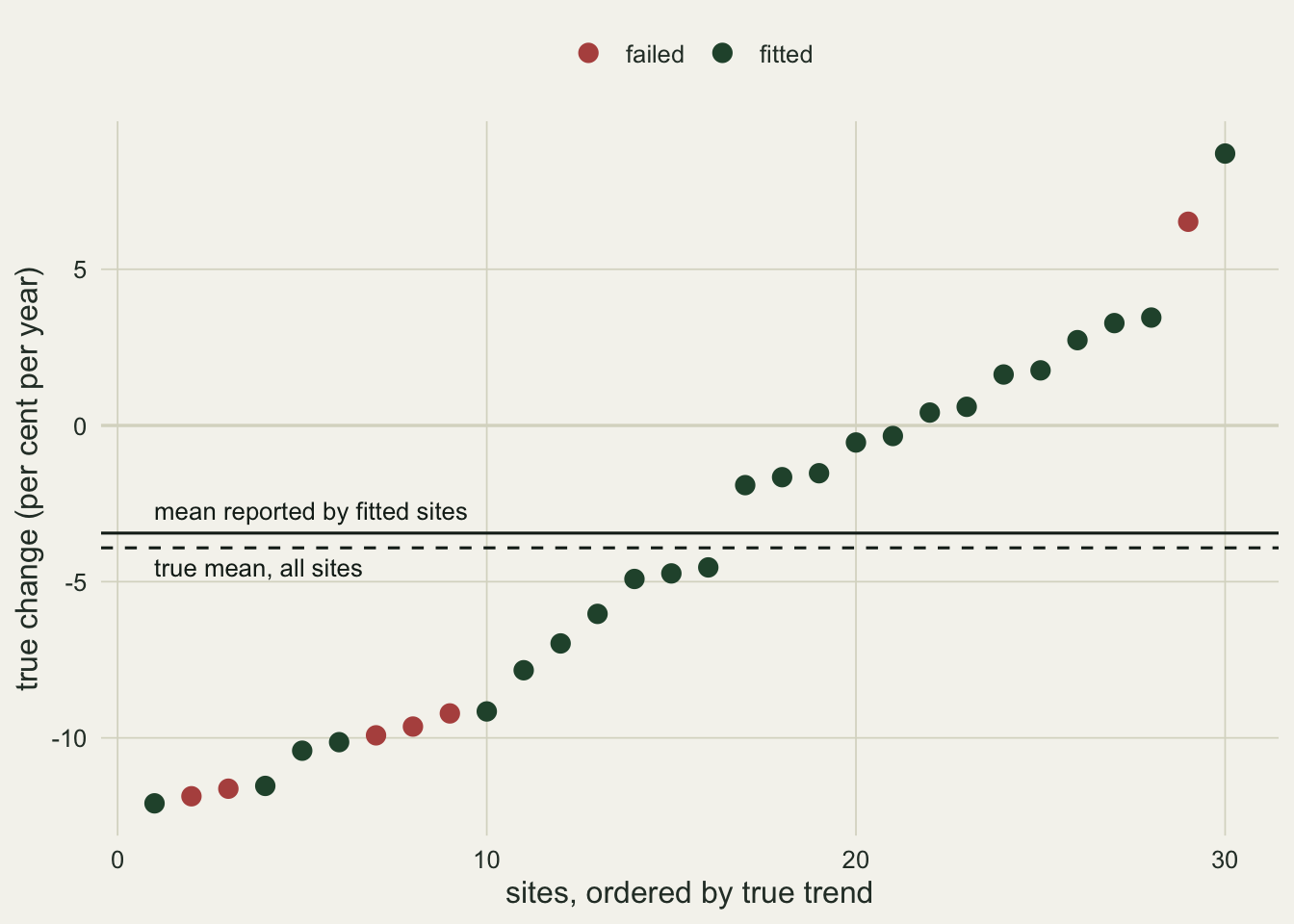
One survey is one draw, and its gap could be luck. For this failure the average gap can be worked out without simulating whole surveys. A site is fitted only if all ten of its counts are above zero, and the chance of that is the product of 1 - exp(-mu) over the ten years. Weight each site’s true trend by that chance, and the weighted mean is the mean over the sites that would be fitted. The chunk below does this for a large sample of sites drawn from the same design; draw_sites() is the design, written once so that the simulation further down can reuse it.

draw_sites <- function(n, anchor_year) {
  level <- exp(rnorm(n, log(10), 0.7))   # expected count in anchor_year
  trend <- rnorm(n, -0.03, 0.08)
  list(mu = exp(outer(years - anchor_year, trend)) * rep(level, each = length(years)),
       true_pct = 100 * (exp(trend) - 1))
}
expected_shift <- function(anchor_year, n = 1e5) {
  s <- draw_sites(n, anchor_year)
  p_fit <- apply(1 - exp(-s$mu), 2, prod)   # chance of no zero in ten years
  c(failed = n_site * mean(1 - p_fit),
    shift  = weighted.mean(s$true_pct, p_fit) - mean(s$true_pct))
}
set.seed(1); expect_start <- expected_shift(anchor_year = 2015)
expect_start

  failed    shift 
3.373400 0.781275 

The design predicts 3.4 failed sites out of 30 in an average survey, and a shift of 0.78 percentage points per year in the mean true trend once they are dropped. That shift is a property of the design, not something a simulation has to discover. What a simulation adds is how much it varies from one survey to the next. The chunk below runs 2000 surveys and uses the closed form of the regression slope instead of lm(), which gives the same number much faster; the first stopifnot() line checks that on site 1, and the last one checks the simulation against the prediction.

slope_fast <- function(y, x) sum((x - mean(x)) * (y - mean(y))) / sum((x - mean(x))^2)
stopifnot(all.equal(slope_fast(log(by_site[["S01"]]$count), years),
                    coef(lm(log(count) ~ year, by_site[["S01"]]))[["year"]]))
one_survey <- function(anchor_year) {
  s <- draw_sites(n_site, anchor_year)
  counts <- matrix(rpois(length(s$mu), s$mu), nrow = length(years))
  fails <- colSums(counts == 0) > 0
  est_pct <- 100 * (exp(apply(log(counts[, !fails, drop = FALSE]), 2,
                              slope_fast, x = years)) - 1)
  c(selection = mean(s$true_pct[!fails]) - mean(s$true_pct),
    reported  = mean(est_pct) - mean(s$true_pct),
    n_failed  = sum(fails), true_mean = mean(s$true_pct))
}
set.seed(99); n_rep <- 2000
gap <- replicate(n_rep, one_survey(anchor_year = 2015))
mc_se <- apply(gap, 1, sd) / sqrt(n_rep)
round(rbind(mean = rowMeans(gap), mc_se = mc_se), 3)

      selection reported n_failed true_mean
mean      0.770    0.827    3.328    -2.647
mc_se     0.014    0.023    0.039     0.031

mean(gap["selection", ] > 0)

[1] 0.8985

stopifnot(abs(mean(gap["selection", ]) - expect_start[["shift"]]) < 3 * mc_se[["selection"]])

The simulated surveys agree with the prediction: an average of 3.3 sites failed, and dropping them raised the mean trend by 0.77 percentage points per year (Monte Carlo standard error 0.014). The shift was upward in 90 per cent of the surveys, so a single survey usually shows it, though not every time. The mean of the reported estimates sat 0.83 points above the truth (standard error 0.023). The true mean decline averaged 2.65 per cent per year, so dropping the failed sites alone hid 29 per cent of it, without an error or a warning anywhere in the script.

Flagging the failures does not remove that shift; it makes it visible. Adding one before taking the log, log(count + 1), makes the error go away but not the problem, because the trend it reports then depends on the constant you added. The fix for this particular failure is a model that accepts zero counts, such as a Poisson GLM, and Poisson and negative binomial GLMs in R shows how. With glm(count ~ year, family = poisson) in place of the log-count regression, every site returns a trend:

glm_pct <- function(d) {
  fit <- glm(count ~ year, family = poisson, data = d)
  100 * (exp(coef(fit)[["year"]]) - 1)
}
pct_glm <- map_dbl(by_site, possibly(glm_pct, otherwise = NA_real_))
c(sites_fitted = sum(!is.na(pct_glm)), mean_trend = mean(pct_glm))

sites_fitted   mean_trend 
   30.000000    -4.508713 

All 30 sites are fitted, and the mean trend is -4.5 per cent per year against the true -3.9. In this survey the estimate misses on the other side, and one survey cannot say which method is closer on average. What changed is that no site is missing from the mean, so there is no selection left to lean it one way.

What to check in your own data

Before trusting a per-site table, count its rows and compare the count with the number of sites you surveyed. stopifnot(NROW(result) == length(unique(data$site))) is one line, and it catches the dropped sites, the tied sites counted twice and the empty filter. Write NROW(), in capitals: it also counts the elements of a plain vector, where nrow() returns NULL, the comparison gives logical(0) and stopifnot() quietly passes.

Run the function on the site you would least like to analyse by hand: the one with the fewest visits, the most zeros or a single year of data. If it gives a sensible answer there, the loop over the easy sites is unlikely to surprise you. Writing that check down as a test is covered in Testing your analysis code.

When a site fails, keep it as a named NA and look at the failed sites as a group before averaging anything. Compare their counts, their number of years and their habitat with the sites that were fitted. If the failures lean one way, the summary leans the other way.

Where a result should be one number per site, say so with vapply(..., numeric(1)) or map_dbl(), so that a site that breaks the rule stops the script instead of reshaping the output.

Honest limits

The direction of the shift comes from how the survey was simulated: each site entered the scheme at its own abundance and then followed its own trend, so the declining sites were the ones most likely to reach zero. That is a common way for monitoring schemes to start, but it is a choice. The chunk below repeats the calculation with each site’s abundance fixed at the middle of the period instead, so that a declining site and an increasing one reach their lowest count equally far from the middle.

set.seed(1); expect_mid <- expected_shift(anchor_year = mean(years))
rbind(start = expect_start, middle = expect_mid)

         failed      shift
start  3.373400 0.78127503
middle 1.996755 0.06180194

stopifnot(expect_mid[["shift"]] > 0, expect_mid[["shift"]] < expect_start[["shift"]] / 10)

With that design 2.0 sites fail in an average survey, and dropping them shifts the mean trend by 0.06 percentage points per year: less than a tenth of the 0.78 when the sites were anchored at the start, though still above zero. It stays positive because the average site in this design is declining, so among the steepest trends, the ones most likely to reach zero at one end of the period, declines outnumber increases. The general lesson does not depend on the design: failures are rarely a random subset, so their direction has to be looked at, not assumed.

References

• R Core Team 2024 R documentation: lapply, sapply and vapply and seq_along.
• Wickham H, Henry L 2023 purrr package documentation: map() and map_dbl(), possibly() and list_c().
• Wickham H, Francois R, Henry L, Muller K, Vaughan D 2023 dplyr 1.1.4 package documentation: group_by() and summarise().
• Wickham H 2019 Advanced R, 2nd edition, Chapman and Hall/CRC (ISBN 978-0-8153-8457-1; DOI 10.1201/9781351201315): section 5.3.1 on loop pitfalls and section 9.2.1 on sapply() and vapply().

Related tutorials

• Summarising ecological data by group
• Debugging and defensive R code
• Testing your analysis code
• Turning your code into an R package