library(dplyr)
library(ggplot2)

te_paper  <- "#f5f4ee"
te_ink    <- "#16241d"
te_forest <- "#275139"
te_rust   <- "#b5534e"
te_gold   <- "#c9b458"
te_line   <- "#dad9ca"
te_canvas <- theme(plot.background  = element_rect(fill = te_paper, colour = NA),
panel.background = element_rect(fill = te_paper, colour = NA))Recoding field data in R: ifelse, if_else, case_when
R
dplyr
data wrangling
data cleaning
missing data
ecology tutorial
Turning tree diameters into size classes in R: why case_when order matters, where the missing values end up, and what ifelse does to dates and factors.
A tree inventory records one number per stem: the diameter at breast height, in centimetres. The report wants something coarser. The protocol says a stem under 10 cm is a sapling, 10 to under 25 cm is a pole, 25 to under 50 cm is a mature tree and anything from 50 cm up is a large tree, and the table of counts per class is the first thing anybody reads. Turning a measurement into classes like this is called recoding, and in R it is one line of case_when(), if_else() or ifelse(). The line runs, the table looks like a table, and the counts can still be wrong.
This post recodes one simulated inventory in several ways and measures what each mistake does to the counts. It stays with numbers turned into classes. Recoding text by a lookup table is the subject of Cleaning species names before you count, the difference between a blank cell and NA is in Reading field data into R, and parsing dates is in Dates and times in ecological data; this post links to those rather than repeating them.
The short answer
Write the conditions of a case_when() from the most specific to the most general, or write each class as a closed interval so the order cannot matter. Deal with missing values in their own line before any catch-all, because a catch-all takes them too. Use dplyr::if_else() rather than base ifelse() when the result is a date or a factor, and check the class of what comes back. When the classes are intervals, cut() with explicit breaks is often the clearest tool, but check which side of each break a value exactly on the boundary goes to. And after every recode, look at the smallest and largest raw value inside each class.
A simulated inventory
The data are simulated, with a fixed seed so every number below is reproducible: 400 stems from 5 cm up, diameters recorded to the nearest centimetre as some inventory sheets do, and 20 stems with no diameter at all (a stem behind a fence, a multi-stemmed hazel nobody agreed how to measure).
set.seed(1013)
n_stem <- 400
n_unmeasured <- 20

stems <- data.frame(
  stem = sprintf("T%03d", 1:n_stem),
  dbh  = 5 + round(rgamma(n_stem, shape = 2, rate = 0.1))
)
dbh_simulated <- stems$dbh   # kept aside: the sheet never shows these for the lost stems
stems$dbh[sample(n_stem, n_unmeasured)] <- NA

summary(stems$dbh)
Min. 1st Qu. Median Mean 3rd Qu. Max. NA's
6.00 15.00 22.00 25.55 33.00 84.00 20 The diameters run from 6 to 84 cm with a median of 22 cm. Half of the measured stems lie between 15 and 33 cm, with few saplings and a long tail of big trees. That hump-shaped distribution fits a stand that regenerated mostly at one time, not an uneven-aged wood, where the thinnest stems are the most numerous.
case_when() stops at the first true condition
case_when() reads its conditions from top to bottom, and each stem gets the value of the first condition that is true for it. The later lines are never consulted for that stem. The dplyr documentation says so, and the chunk below checks it on the single value 30:
stopifnot(case_when(30 > 10 ~ "pole", 30 > 25 ~ "mature") == "pole")Now the recode as it is often first written, with the thresholds in the order they appear in the protocol, lowest first:
stems <- stems |>
  mutate(class_lowest_first = case_when(
    dbh >= 10 ~ "pole",
    dbh >= 25 ~ "mature",
    dbh >= 50 ~ "large",
    dbh < 10  ~ "sapling"
  ))
count(stems, class_lowest_first)
class_lowest_first n
1 pole 351
2 sapling 29
3 <NA> 20There is no mature tree and no large tree in the whole wood. A stem of 60 cm satisfies dbh >= 10, so it becomes a pole and the two lines below that one never see it. Put the most specific condition first and the same four lines give the protocol’s classes:
stems <- stems |>
  mutate(size_class = case_when(
    dbh >= 50 ~ "large",
    dbh >= 25 ~ "mature",
    dbh >= 10 ~ "pole",
    dbh < 10  ~ "sapling"
  ))
count(stems, size_class)
size_class n
1 large 23
2 mature 137
3 pole 191
4 sapling 29
5 <NA> 20n_wrong <- sum(stems$class_lowest_first != stems$size_class, na.rm = TRUE)
n_measured <- sum(!is.na(stems$dbh))
d <- which(stems$class_lowest_first != stems$size_class)
stopifnot(all(stems$class_lowest_first[d] == "pole"),
identical(d, which(stems$size_class %in% c("mature", "large"))))The two versions disagree on 160 of the 380 measured stems, 42.1 per cent of them, and every one of those was a mature or large tree filed as a pole. Nothing warned.
The share is not a property of the code. With the lowest threshold first, every stem of 25 cm or more becomes a pole, so the share misclassified is simply the share of stems in the two higher classes. For this simulated stand it can be worked out without the data: a diameter is 25 cm or more when the rounded gamma draw is 20 or more, that is, when the draw itself is at least 19.5.
p_big <- pgamma(19.5, shape = 2, rate = 0.1, lower.tail = FALSE)
p_big
[1] 0.4197085The expected share is 42.0 per cent, and the 42.1 per cent above is what one draw of 400 stems gave. In a stand with few trees of 25 cm or more, the same code would move few stems; in a stand of mostly big trees it would move most of them.
The alternative that does not depend on order at all is to write each class as a closed interval, dbh >= 10 & dbh < 25 ~ "pole", so that no stem can satisfy two lines. It is longer, and it is the version to prefer when somebody else will edit the code later.
Missing values fall through to the catch-all
Most recodes end with a line that catches everything left over. In dplyr 1.1.0 and later that is the .default argument; older code writes TRUE ~ "sapling", which does the same. It is tempting for the smallest class, because anything not caught above must be small.
stems <- stems |>
  mutate(class_catch_all = case_when(
    dbh >= 50 ~ "large",
    dbh >= 25 ~ "mature",
    dbh >= 10 ~ "pole",
    .default  = "sapling"
  ))
count(stems, class_catch_all)
class_catch_all n
1 large 23
2 mature 137
3 pole 191
4 sapling 49The NA row has gone, and the saplings have grown by exactly the number of unmeasured stems. For a stem with no diameter, dbh >= 50 is NA, not FALSE, and case_when() treats an NA condition as not true, moves on, and ends up at the catch-all. The documentation for .default states this directly, and it is the behaviour the next chunk guards, together with what happens when there is no catch-all:
stopifnot(
  case_when(NA_real_ > 10 ~ "pole", .default = "sapling") == "sapling",
  is.na(case_when(NA_real_ > 10 ~ "pole"))
)

share_true  <- mean(stems$size_class == "sapling", na.rm = TRUE)
share_catch <- mean(stems$class_catch_all == "sapling")
n_moved <- sum(is.na(stems$dbh) & stems$class_catch_all == "sapling")
n_moved_small <- sum(is.na(stems$dbh) & dbh_simulated < 10)
20 stems of unknown size are now saplings. The sapling share of the measured stems is 7.6 per cent; in the catch-all version it is 12.2 per cent, and it looks like a finding about regeneration rather than a gap on the data sheet. Because the data are simulated, we can look up the diameters those stems had before they were lost: only 1 of the 20 had been under 10 cm. The catch-all did not guess the class of an unknown stem; it filed all of them in the one class that happened to be written last.
The fix is one line at the top, or no catch-all at all:
stems <- stems |>
  mutate(class_na_first = case_when(
    is.na(dbh) ~ NA,
    dbh >= 50  ~ "large",
    dbh >= 25  ~ "mature",
    dbh >= 10  ~ "pole",
    .default   = "sapling"
  ))
stopifnot(identical(stems$class_na_first, stems$size_class))
With is.na(dbh) ~ NA first, the catch-all only sees measured stems, and the result is identical to the four-condition version. The recode in size_class needed no such line because it had no catch-all: a stem that matched nothing got NA, which is what an unmeasured stem should get. dplyr 1.2.0 added a third option, .unmatched = "error", which stops with an error instead of filling in when a value matches no line (the dplyr changelog). It is not in dplyr 1.1.4, the version this post was written with, so it is not run here.
class_levels <- c("sapling", "pole", "mature", "large", "not measured")
version_levels <- c("lowest threshold first", "catch-all for saplings", "highest threshold first")

tally <- bind_rows(
  count(stems, class = class_lowest_first) |> mutate(version = version_levels[1]),
  count(stems, class = class_catch_all)    |> mutate(version = version_levels[2]),
  count(stems, class = size_class)         |> mutate(version = version_levels[3])
) |>
  mutate(class = coalesce(class, "not measured"))

# every class in every version, with 0 where a version has no stems in it
tally <- expand.grid(class = class_levels, version = version_levels,
                     stringsAsFactors = FALSE) |>
  left_join(tally, by = c("class", "version")) |>
  mutate(n = coalesce(n, 0L),
         class = factor(class, levels = class_levels),
         version = factor(version, levels = version_levels))

ggplot(tally, aes(class, n, fill = version)) +
  geom_col(position = position_dodge(width = 0.8), width = 0.78) +
  geom_text(aes(label = n), position = position_dodge(width = 0.8),
            vjust = -0.4, size = 3, colour = te_ink) +
  scale_fill_manual(values = c(te_rust, te_gold, te_forest)) +
  scale_y_continuous(expand = expansion(mult = c(0, 0.08))) +
  labs(x = NULL, y = "number of stems", fill = NULL) +
  theme_minimal(base_size = 12) + te_canvas +
  theme(legend.position = "top", panel.grid.minor = element_blank(),
        panel.grid.major.x = element_blank(),
        text = element_text(colour = te_ink))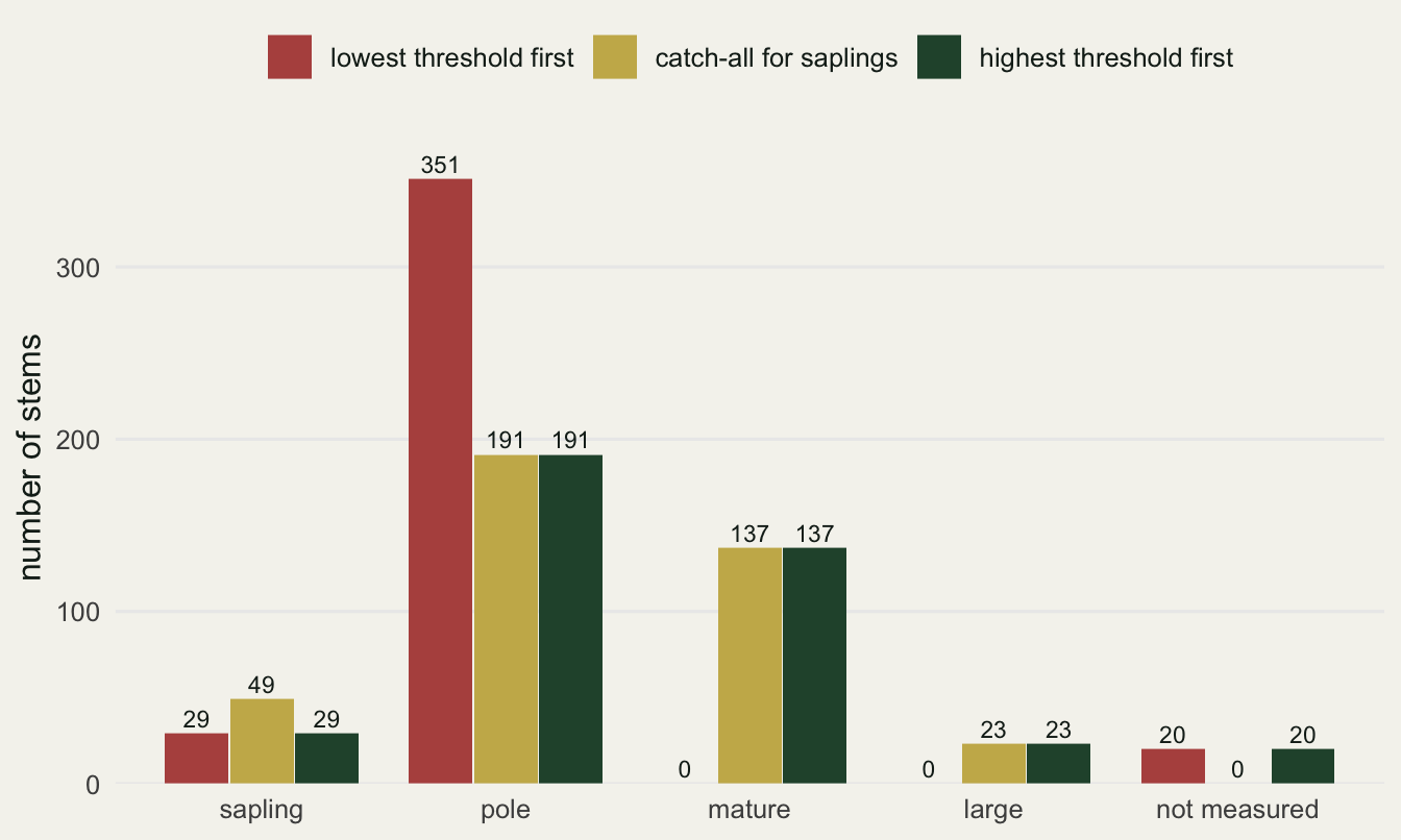
ifelse() and if_else()
For two classes, ifelse() from base R and if_else() from dplyr look interchangeable, and for a character result they are. The difference shows with dates. Suppose ten plots were each planned for a visit a week apart, the visit date was written on the sheet, and two sheets have no date. Filling a missing visit date with the planned one is a common repair:
plots <- data.frame(
  plot    = sprintf("P%02d", 1:10),
  planned = as.Date("2025-05-05") + 7 * (0:9)
)
plots$visited <- plots$planned + sample(0:3, 10, replace = TRUE)
plots$visited[c(4, 9)] <- NA

filled_base  <- ifelse(is.na(plots$visited), plots$planned, plots$visited)
filled_dplyr <- if_else(is.na(plots$visited), plots$planned, plots$visited)
head(filled_base, 3)
[1] 20214 20223 20230head(filled_dplyr, 3)[1] "2025-05-06" "2025-05-15" "2025-05-22"stopifnot(is.numeric(filled_base), !inherits(filled_base, "Date"),
inherits(filled_dplyr, "Date"))ifelse() returned 20214 where the sheet said 2025-05-06. The help page for ifelse() explains why: the result takes its attributes, including the class, from the condition, which is a plain logical vector, so the Date class is dropped and the day count underneath is all that remains. if_else() keeps the class of true and false. The same thing happens with a factor, where ifelse() returns the level codes:
habitat <- factor(c("wood", "fen", "meadow", "fen"))
ifelse(habitat == "fen", "wetland", habitat)
[1] "3" "wetland" "2" "wetland"if_else(habitat == "fen", "wetland", habitat)[1] "wood" "wetland" "meadow" "wetland"stopifnot(is.character(if_else(habitat == "fen", "wetland", habitat)),
is.character(if_else(habitat == "fen", "meadow", habitat)))if_else() returns the labels, as text: a text value and a factor combine to text, whether or not the text is one of the factor’s levels (the second line of the check uses “meadow”, which is). Wrap the result in factor() if you need a factor again.
if_else() is also strict where ifelse() is not: it refuses to combine a number and a text value, and it has a missing argument for the case where the condition itself is NA.
stopifnot(inherits(try(if_else(TRUE, "sapling", 1), silent = TRUE), "try-error"))

stems <- stems |>
  mutate(tree_or_sapling = if_else(dbh >= 10, "tree", "sapling",
                                   missing = "not measured"))
count(stems, tree_or_sapling)
tree_or_sapling n
1 not measured 20
2 sapling 29
3 tree 351stopifnot(sum(stems$tree_or_sapling == "not measured") == n_unmeasured)Without missing, those 20 stems would be NA, which is also honest. What if_else() never does is put them in one of the two classes.
cut() and the stem on the boundary
When the classes are intervals on one measurement, cut() states them as a vector of breaks and cannot get the order wrong. It has its own question to answer: which class does a stem of exactly 10 cm belong to? The default, right = TRUE, closes each interval on the right, so the intervals are (0, 10], (10, 25] and so on, and 10 goes into the lower class.
breaks <- c(0, 10, 25, 50, Inf)
size_labels <- c("sapling", "pole", "mature", "large")

stems <- stems |>
  mutate(cut_right = cut(dbh, breaks, labels = size_labels),
         cut_left  = cut(dbh, breaks, labels = size_labels, right = FALSE))

stopifnot(cut(10, breaks) == "(0,10]", cut(10, breaks, right = FALSE) == "[10,25)")

n_boundary <- sum(stems$dbh %in% c(10, 25, 50))
n_differ_right <- sum(as.character(stems$cut_right) != stems$size_class, na.rm = TRUE)
n_differ_left  <- sum(as.character(stems$cut_left)  != stems$size_class, na.rm = TRUE)
c(on_a_boundary = n_boundary, default_differs = n_differ_right,
  right_false_differs = n_differ_left)
on_a_boundary default_differs right_false_differs
21 21 0 differs <- which(as.character(stems$cut_right) != stems$size_class)
stopifnot(n_differ_left == 0,
identical(differs, which(stems$dbh %in% c(10, 25, 50))))The protocol says “10 to under 25 cm”, which is the interval [10, 25), so right = FALSE is the setting that matches it, and it agrees with the case_when() version on every measured stem. The default puts 21 stems into the class below, and they are precisely the 21 stems recorded at 10, 25 or 50 cm. That is 5.5 per cent of the measured stems. Diameters rounded to whole centimetres make boundary values frequent: with every value an integer, each break is a value that real records take. How often a stem lands exactly on a break depends on the recording resolution, and for the simulated stand it can be worked out:
breaks_on_draw <- c(10, 25, 50) - 5   # the breaks on the scale of the gamma draw
share_on_break <- function(step) {    # step: recording resolution in cm
  sum(pgamma(breaks_on_draw + step / 2, 2, 0.1) -
      pgamma(breaks_on_draw - step / 2, 2, 0.1))
}
on_break <- c(whole_cm = share_on_break(1), tenth_cm = share_on_break(0.1))
on_break
whole_cm tenth_cm
0.062355875 0.006239227 Recorded to the whole centimetre, 6.2 per cent of the stems are expected on a break; recorded to 0.1 cm, 0.62 per cent, a tenth as many. How many stems this affects depends on how coarsely the sheet records diameter; which way the boundary stems go does not.
cut() also leaves one end of the breaks open, and a value equal to that break becomes NA: with the default right = TRUE it is the lowest break, with right = FALSE the highest. With breaks from 0 to Inf and diameters of 5 cm and more, neither can happen here. For cover classes from 0 to 100 per cent, the default loses every bare quadrat and right = FALSE loses every quadrat at full cover. include.lowest = TRUE closes the open end in both cases (the name says “lowest”, but with right = FALSE it closes the highest break):
cover_breaks <- c(0, 5, 25, 50, 75, 100)
stopifnot(is.na(cut(0, cover_breaks)),
          is.na(cut(100, cover_breaks, right = FALSE)),
          !is.na(cut(0, cover_breaks, include.lowest = TRUE)),
          !is.na(cut(100, cover_breaks, right = FALSE, include.lowest = TRUE)))
Missing values stay missing in cut(), which is the behaviour you want:
stopifnot(is.na(cut(NA_real_, breaks)))What to check in your own data
The one check that would have caught every class mistake above is a grouped summary of the raw measurement inside each new class. A class that holds values outside its own range has been filled from the wrong line.
stems |>
  group_by(class_lowest_first) |>
  summarise(n = n(), smallest = min(dbh), largest = max(dbh))
# A tibble: 3 × 4
class_lowest_first n smallest largest
<chr> <int> <dbl> <dbl>
1 pole 351 10 84
2 sapling 29 6 9
3 <NA> 20 NA NAstems |>
group_by(class_catch_all) |>
summarise(n = n(), smallest = min(dbh), largest = max(dbh))# A tibble: 4 × 4
class_catch_all n smallest largest
<chr> <int> <dbl> <dbl>
1 large 23 50 84
2 mature 137 25 49
3 pole 191 10 24
4 sapling 49 NA NAstems |>
group_by(cut_right) |>
summarise(n = n(), smallest = min(dbh), largest = max(dbh))# A tibble: 5 × 4
cut_right n smallest largest
<fct> <int> <dbl> <dbl>
1 sapling 38 6 10
2 pole 190 11 25
3 mature 133 26 50
4 large 19 52 84
5 <NA> 20 NA NAprotocol_ok <- with(stems, all(
(size_class == "sapling" & dbh < 10) |
(size_class == "pole" & dbh >= 10 & dbh < 25) |
(size_class == "mature" & dbh >= 25 & dbh < 50) |
(size_class == "large" & dbh >= 50), na.rm = TRUE))
stopifnot(protocol_ok, sum(is.na(stems$size_class)) == sum(is.na(stems$dbh)))
pole_max <- max(stems$dbh[stems$class_lowest_first == "pole"], na.rm = TRUE)
sapling_max_cut <- max(stems$dbh[stems$cut_right == "sapling"], na.rm = TRUE)Each table shows its own mistake. With the lowest threshold first, the pole class runs up to 84 cm. With the catch-all, the sapling row has NA as its smallest and largest value: min() and max() return NA when any value in the group is missing, and a class of measured stems should have none. With the default cut(), the sapling class reaches 10 cm, which the protocol calls a pole. For size_class every stem sits inside its protocol limits and the missing values line up with the missing diameters, which is what the final stopifnot() checks. The grouping itself is covered in Summarising ecological data by group.
Beyond that, four things are quick to check on any recode. Count the missing values before and after: sum(is.na(dbh)) should equal the number of stems whose class is NA (or “not measured”), and if it is smaller, a catch-all has absorbed some. Put a value that sits exactly on each boundary through the code and read which class it lands in; with whole-number measurements, some real records sit there. Run class() on the result when the input was a date or a factor. And if your conditions overlap, read them in order as the function does, from the top, and ask of a big value which line it meets first.
None of these checks can tell you whether the protocol’s boundaries are sensible for the question; that is an ecological decision, and Size-class boundaries in a matrix population model shows how much it can change a result. The checks only tell you that the code does what the protocol says. The chapter on logical vectors in Wickham, Cetinkaya-Rundel and Grolemund (2023) covers if_else() and case_when() with more examples, and the reference pages for case_when() and if_else() are the place to confirm the rules for the version you have installed.
References
- Wickham H, Cetinkaya-Rundel M, Grolemund G 2023 R for Data Science, 2nd edn. O’Reilly (ISBN 978-1-492-09740-2; free online at https://r4ds.hadley.nz)
- Wickham H, Francois R, Henry L, Muller K, Vaughan D 2023 dplyr: A Grammar of Data Manipulation. R package (written with version 1.1.4; https://dplyr.tidyverse.org)