library(ggplot2)
library(patchwork)

te_paper  <- "#f5f4ee"
te_ink    <- "#16241d"
te_body   <- "#2c3a31"
te_forest <- "#275139"
te_rust   <- "#b5534e"
te_gold   <- "#c9b458"
te_line   <- "#dad9ca"

theme_datasheet <- function() {
  theme_minimal(base_size = 12) +
    theme(plot.background  = element_rect(fill = te_paper, colour = NA),
          panel.background = element_rect(fill = te_paper, colour = NA),
          panel.grid.major = element_line(colour = te_line, linewidth = 0.3),
          panel.grid.minor = element_blank(),
          text             = element_text(colour = te_body),
          plot.title       = element_text(colour = te_ink, face = "bold"),
          plot.subtitle    = element_text(colour = te_body),
          axis.text        = element_text(colour = te_body),
          strip.text       = element_text(colour = te_ink, face = "bold"))
}
rule_cols <- c("equal width" = te_rust, "quantile" = te_forest)Size-class boundaries in a matrix population model
R
matrix models
demography
population dynamics
simulation
ecology tutorial
Equal-width size classes can turn a declining population into a stable or growing one. In R: how quantile boundaries protect lambda in a matrix model.
A perennial herb is tagged in a grassland reserve: 120 rosettes, each measured once in June, found again the next June and scored as dead, alive at a new size, or alive with a count of seedlings around it. The data are individuals with a continuous size, and the matrix model that will be built from them needs classes. Somebody has to decide where the boundaries go, and the usual choice is the one that looks most neutral: split the size axis into equal-width classes, as many as seems reasonable, and count transitions between them.
Building an integral projection model states the problem in one sentence and moves on: a plant, a fish or a tortoise has a continuous size, “and where you put the class boundaries changes the answer”. That post keeps size continuous and never measures how much the answer changes. This one measures it, with a matrix model fitted to simulated individuals from a known size kernel, so that the true growth rate is known to four decimals.
The nearest post on the site points the other way. The second trap of eviction and mesh size in an IPM, mesh size, discretises a kernel that is known exactly; the only error is quadrature error, and the advice is that refining the mesh converges it, so more bins are always at least as good. Here the kernel is not known. Every transition in the matrix is estimated from the same individuals the classes are cut from, so each extra class divides a fixed sample more finely, and the direction of that advice reverses: past a point, more classes make lambda worse, and the classes the equal-width rule adds are exactly the ones nobody lives in.
The closest measurement on the site is check four of checking a matrix population model. It bootstraps lambda at four levels of field effort and reports the share of resampled matrices that grow, which is the measure used below under another name. It does that at a fixed four-stage scheme with the stages given, and its parametric bootstrap is centred on the matrix that generated the data. Check four showed that the interval on lambda is wide. This post shows that the class boundary rule is one of the things that sets that width, and that it also puts a bias inside it, which check four, with its stages given and no class boundaries to choose, could not show.
None of this is new. Vandermeer (1978) posed the choice of category size in a stage projection matrix as a balance between two errors, which this post calls sampling error and distribution error: errors of estimation, from estimating each transition out of the few individuals in a class that is too narrow, and errors of distribution, from treating individuals of different sizes inside a class that is too wide as identical; he also suggested an approximate way to balance them. Moloney (1986) revised and generalised that algorithm. Picard, Ouedraogo and Bar-Hen (2010) returned to the choice of classes for size projection matrices, and Salguero-Gomez and Plotkin (2010) showed that matrix dimension biases the elasticities that comparative studies compare. This post is a demonstration of those papers rather than a finding of its own. What it measures is the price: how often the boundary rule flips the verdict on whether the population is growing, and how much of the price a one-line rule, class boundaries at sample quantiles, recovers without running Moloney’s algorithm at all.
A plant with a continuous size and a known lambda
The plant lives on a size axis from 0 to 12 (a log leaf length, say). Survival is logistic in size, next year’s size is a linear function of this year’s with normal scatter, the expected number of recruits rises exponentially with size, and recruits arrive with a normal size of their own. These are the building blocks of the integral projection model post, with flowering and recruit number folded into one expected fecundity and with constants fixed before anything below was run. The truth is the dominant eigenvalue of that kernel discretised by the midpoint rule on 400 bins, which is the known-kernel problem of the mesh post, solved well enough to be a reference.
z_lo <- 0
z_hi <- 12
surv_fun <- function(z) plogis(-1.15 + 0.42 * z)
grow_mu  <- function(z) 1.05 + 0.78 * z
grow_sd  <- 0.90
fec_fun  <- function(z) exp(-3.05 + 0.42 * z)
rec_mu   <- 1.5
rec_sd   <- 0.60

kernel_parts <- function(m_bin) {
  h_bin <- (z_hi - z_lo) / m_bin
  mesh  <- z_lo + (seq_len(m_bin) - 0.5) * h_bin
  g_mat <- outer(mesh, mesh, function(zp, z) dnorm(zp, grow_mu(z), grow_sd))
  g_mat <- sweep(g_mat, 2, colSums(g_mat), "/")
  c_vec <- dnorm(mesh, rec_mu, rec_sd)
  c_vec <- c_vec / sum(c_vec)
  list(mesh = mesh, h = h_bin,
       P = sweep(g_mat, 2, surv_fun(mesh), "*"),
       F = outer(c_vec, fec_fun(mesh)))
}

lam_and_elas <- function(p_mat, f_mat) {
  a_mat <- p_mat + f_mat
  e_r <- eigen(a_mat)
  e_l <- eigen(t(a_mat))
  i_r <- which.max(Re(e_r$values))
  i_l <- which.max(Re(e_l$values))
  lam <- Re(e_r$values[i_r])
  w_r <- abs(Re(e_r$vectors[, i_r]))
  v_l <- abs(Re(e_l$vectors[, i_l]))
  e_fec <- sum(f_mat * outer(v_l, w_r)) / (lam * sum(v_l * w_r))
  c(lambda = lam, e_fec = e_fec)
}

kern_400  <- kernel_parts(400)
kern_800  <- kernel_parts(800)
truth_400 <- lam_and_elas(kern_400$P, kern_400$F)
truth_800 <- lam_and_elas(kern_800$P, kern_800$F)
lam_true  <- truth_400[["lambda"]]
efec_true <- truth_400[["e_fec"]]
mesh_gap  <- abs(truth_800[["lambda"]] - lam_true)
decline   <- 100 * (1 - lam_true)

w_stab <- Re(eigen(kern_400$P + kern_400$F)$vectors[, 1])
w_stab <- w_stab / sum(w_stab)
stab_q <- function(p) kern_400$mesh[which(cumsum(w_stab) >= p)[1]]
z_q50  <- stab_q(0.50)
z_q99  <- stab_q(0.99)
The true growth rate is 0.8006: a population shrinking by 20 per cent a year, which is not a marginal case. Doubling the mesh to 800 bins moves it by \(2.14 \times 10^{-7}\), so the reference is settled. Half of the stable population is smaller than 2.80 and 99 per cent is smaller than 7.84, which leaves the upper third of the size axis almost empty. That emptiness is ordinary: an axis is drawn to hold the largest plant anyone has seen, and most plants are small.
Each simulated study draws n plants from the stable size distribution, follows them for one year through the same survival, growth and recruitment functions (growth and recruit size are drawn from the normal truncated to the axis, which is what the renormalised kernel assumes), cuts the size axis into k classes, and builds the matrix from counts. Each column is the fate of the plants that started in that class: the share that survived into each class plus the number of recruits they produced landing in each class, both divided by the number of plants that started there. Two boundary rules are compared. Equal width splits 0 to 12 into k equal pieces. Quantile puts the inner boundaries at the sample quantiles of this year’s sizes, so each class starts with about n over k plants.
draw_sizes <- function(n) {
  sample(kern_400$mesh, n, replace = TRUE, prob = w_stab) +
    runif(n, -kern_400$h / 2, kern_400$h / 2)
}
rtrunc_norm <- function(n, mu, s) {
  p_lo <- pnorm(z_lo, mu, s)
  p_hi <- pnorm(z_hi, mu, s)
  qnorm(p_lo + runif(n) * (p_hi - p_lo), mu, s)
}
p_breed <- 0.25
follow_year <- function(z, fec_type = "poisson") {
  n <- length(z)
  alive  <- runif(n) < surv_fun(z)
  z_next <- rtrunc_norm(sum(alive), grow_mu(z[alive]), grow_sd)
  n_rec <- if (fec_type == "poisson") {
    rpois(n, fec_fun(z))
  } else {
    (runif(n) < p_breed) * rnbinom(n, size = 1, mu = fec_fun(z) / p_breed)
  }
  list(z = z, alive = alive, z_next = z_next, n_rec = n_rec,
       rec_z = rtrunc_norm(sum(n_rec), rec_mu, rec_sd))
}

stage_cut <- 3
tol_one   <- 1e-8
class_breaks <- function(z, k, rule) {
  if (rule == "equal width") return(seq(z_lo, z_hi, length.out = k + 1))
  if (rule == "equal width, observed range") {
    brk <- seq(min(z), max(z), length.out = k + 1)
    brk[c(1, k + 1)] <- c(z_lo, z_hi)
    return(brk)
  }
  if (rule == "quantile") {
    return(c(z_lo, quantile(z, seq_len(k - 1) / k, names = FALSE), z_hi))
  }
  small <- z < stage_cut
  k_1 <- max(1, min(k - 1, round(k * mean(small))))
  k_2 <- k - k_1
  b_1 <- quantile(z[small], seq_len(k_1 - 1) / k_1, names = FALSE)
  b_2 <- quantile(z[!small], seq_len(k_2 - 1) / k_2, names = FALSE)
  c(z_lo, b_1, stage_cut, b_2, z_hi)
}

loop_type <- function(a_mat) {
  hit <- which(diag(a_mat) >= 1 - tol_one)
  if (length(hit) == 0) return(0)
  reach <- (a_mat > 0) * 1
  diag(reach) <- 1
  for (i in seq_len(ceiling(log2(nrow(a_mat))) + 1)) reach <- (reach %*% reach > 0) * 1
  on_cycle <- vapply(hit, function(j) any(reach[j, -j] * reach[-j, j] > 0), TRUE)
  if (any(on_cycle)) return(3)
  leaves <- vapply(hit, function(j) any(a_mat[-j, j] > 0), TRUE)
  if (any(leaves)) 2 else 1
}

fit_matrix <- function(fl, brk, elas = FALSE) {
  k_cl  <- length(brk) - 1
  cl    <- findInterval(fl$z, brk, all.inside = TRUE)
  n_in  <- tabulate(cl, k_cl)
  cl_nx <- findInterval(fl$z_next, brk, all.inside = TRUE)
  cl_rc <- findInterval(fl$rec_z, brk, all.inside = TRUE)
  p_mat <- matrix(tabulate(cl_nx + (cl[fl$alive] - 1) * k_cl, k_cl^2), k_cl)
  f_mat <- matrix(tabulate(cl_rc + (rep(cl, fl$n_rec) - 1) * k_cl, k_cl^2), k_cl)
  p_mat <- sweep(p_mat, 2, pmax(n_in, 1), "/")
  f_mat <- sweep(f_mat, 2, pmax(n_in, 1), "/")
  d_max <- max(diag(p_mat + f_mat))
  d_type <- loop_type(p_mat + f_mat)
  if (!elas) {
    lam <- max(Re(eigen(p_mat + f_mat, only.values = TRUE)$values))
    return(c(lambda = lam, d_max = d_max, e_fec = NA, d_type = d_type))
  }
  occ <- n_in > 0
  c(lam_and_elas(p_mat[occ, occ, drop = FALSE], f_mat[occ, occ, drop = FALSE]),
    d_max = d_max, d_type = d_type)[c("lambda", "d_max", "e_fec", "d_type")]
}

run_cell <- function(n_rep, n, k, rule, fec_type = "poisson", elas = FALSE) {
  out <- vapply(seq_len(n_rep), function(i) {
    fl <- follow_year(draw_sizes(n), fec_type)
    fit_matrix(fl, class_breaks(fl$z, k, rule), elas)
  }, numeric(4))
  rownames(out) <- c("lambda", "d_max", "e_fec", "d_type")
  out
}
Before any study is run, the stable distribution already says how the two rules will spend 120 plants. The expected number of plants starting in each class follows from the stable distribution alone.
n_show <- 120
k_show <- 20
brk_eq <- seq(z_lo, z_hi, length.out = k_show + 1)
brk_qu <- c(z_lo, sapply(seq_len(k_show - 1) / k_show, stab_q), z_hi)
class_mass <- function(brk) {
  vapply(seq_len(length(brk) - 1), function(j) {
    sum(w_stab[kern_400$mesh >= brk[j] & kern_400$mesh < brk[j + 1]])
  }, 0)
}
cnt_eq <- n_show * class_mass(brk_eq)
cnt_qu <- n_show * class_mass(brk_qu)
n_eq_below1 <- sum(cnt_eq < 1)
n_eq_below3 <- sum(cnt_eq < 3)
cnt_eq_max  <- max(cnt_eq)
cnt_qu_rng  <- range(cnt_qu)
top_k3 <- n_show * sum(w_stab[kern_400$mesh >= 8])
top_k2 <- n_show * sum(w_stab[kern_400$mesh >= 6])
With 20 equal-width classes, 7 of the 20 classes expect fewer than one plant out of 120, and 8 expect fewer than three, while the busiest class expects 19.9. The quantile rule gives every class between 5.2 and 6.7 plants by construction. The equal-width rule does not go wrong because twenty is too many classes for 120 plants; it goes wrong because it spends 7 of its classes on sizes where, on average, not even one plant lives.
rect_df <- rbind(
  data.frame(rule = "equal width", lo = brk_eq[-(k_show + 1)],
             hi = brk_eq[-1], count = cnt_eq),
  data.frame(rule = "quantile", lo = brk_qu[-(k_show + 1)],
             hi = brk_qu[-1], count = cnt_qu))
rect_df$rule <- factor(rect_df$rule, levels = c("equal width", "quantile"))

ggplot(rect_df) +
  geom_rect(aes(xmin = lo, xmax = hi, ymin = 0, ymax = count, fill = rule),
            colour = te_paper, linewidth = 0.4) +
  geom_hline(yintercept = 1, linetype = "dashed", colour = te_ink,
             linewidth = 0.5) +
  facet_wrap(~ rule, ncol = 1) +
  scale_fill_manual(values = rule_cols, guide = "none") +
  scale_x_continuous(breaks = seq(0, 12, by = 2)) +
  labs(x = "size this year", y = "expected plants starting in the class",
       title = "Equal width spends its classes on empty size",
       subtitle = "each bar is one class; dashed line: one plant") +
  theme_datasheet()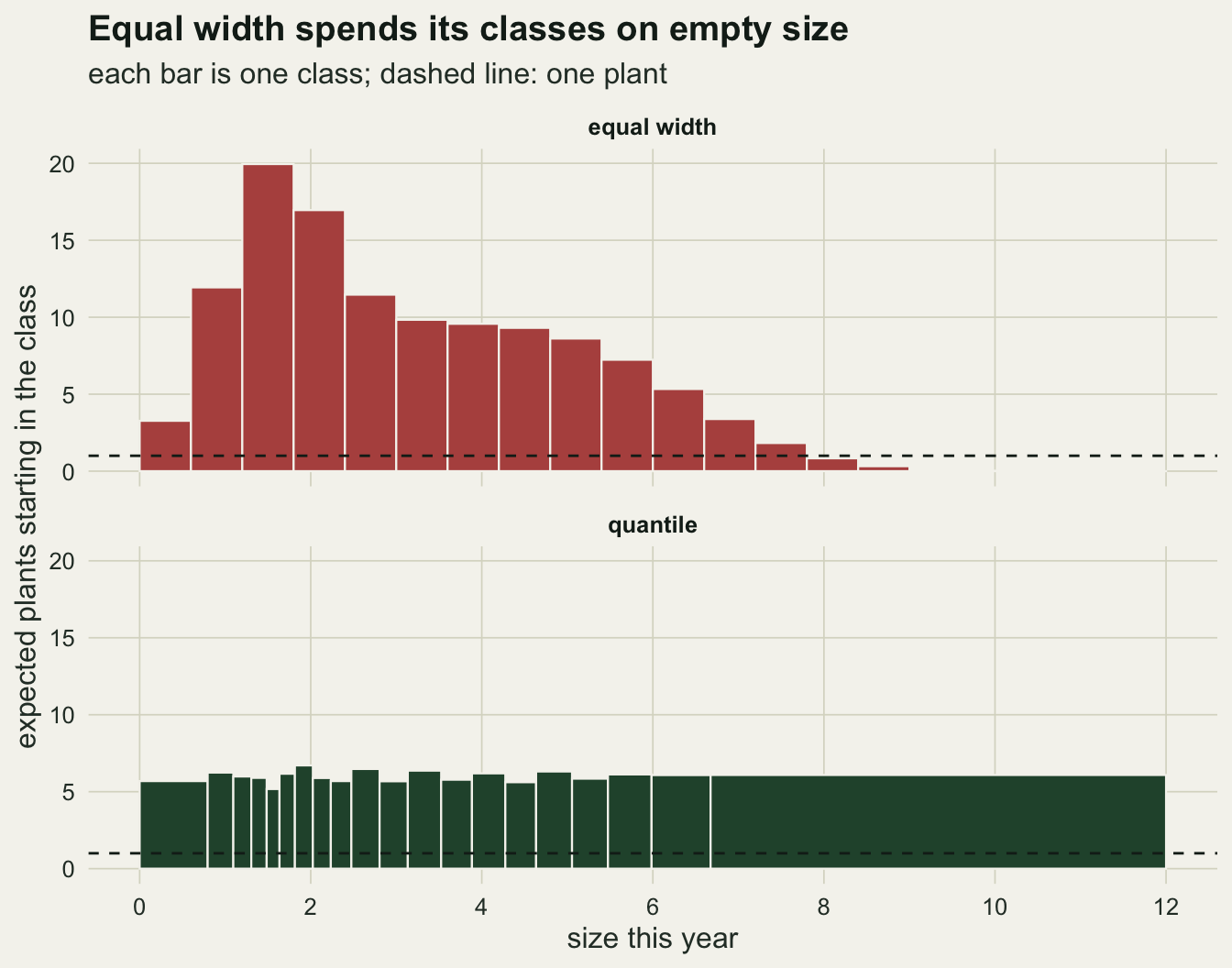
Twenty classes and the sign of the verdict
The number a demographer reports is rarely the root mean square error of lambda. It is whether the population is growing or declining, and that verdict is what the grid below is built to price. Class counts from 2 to 20 are crossed with the two rules and with samples of 120 and 400 plants, and every cell is run as five independent runs of 400 studies, 2000 studies a cell. The replication was fixed before anything ran, so that the Monte Carlo standard error of a rate near five per cent is about half a percentage point.
A verdict can go wrong in two ways here, and they are counted separately. A study is scored as growing when its lambda estimate exceeds one, and as exactly stationary when the estimate equals one to eight decimals. The second category is not a rounding curiosity, as the next section explains.
k_grid    <- c(2, 3, 4, 6, 8, 12, 20)
n_grid    <- c(120, 400)
rules     <- c("equal width", "quantile")
n_run     <- 5
n_per_run <- 400
n_cell    <- n_run * n_per_run

set.seed(20260926)
cells <- expand.grid(k = k_grid, rule = rules, n = n_grid,
                     run = seq_len(n_run), stringsAsFactors = FALSE)
sims <- lapply(seq_len(nrow(cells)), function(i) {
  run_cell(n_per_run, cells$n[i], cells$k[i], cells$rule[i], elas = TRUE)
})
cells$rmse <- vapply(sims, function(m) sqrt(mean((m["lambda", ] - lam_true)^2)), 0)

key_of <- paste(cells$n, cells$rule, cells$k)
pool   <- lapply(split(sims, key_of), function(s) do.call(cbind, s))
grid_tab <- unique(cells[, c("n", "rule", "k")])
grid_tab <- grid_tab[order(grid_tab$n, grid_tab$rule, grid_tab$k), ]
stat_of <- function(f) {
  vapply(paste(grid_tab$n, grid_tab$rule, grid_tab$k), function(key) f(pool[[key]]), 0)
}
grid_tab$rmse   <- stat_of(function(m) sqrt(mean((m["lambda", ] - lam_true)^2)))
grid_tab$bias   <- stat_of(function(m) mean(m["lambda", ]) - lam_true)
grid_tab$bias_se <- stat_of(function(m) sd(m["lambda", ]) / sqrt(ncol(m)))
grid_tab$grow   <- stat_of(function(m) mean(m["lambda", ] > 1 + tol_one))
grid_tab$one    <- stat_of(function(m) mean(abs(m["lambda", ] - 1) <= tol_one))
grid_tab$e_fec  <- stat_of(function(m) mean(m["e_fec", ], na.rm = TRUE))
grid_tab$e_na   <- stat_of(function(m) sum(is.na(m["e_fec", ])))
grid_tab$no_decline <- grid_tab$grow + grid_tab$one

cell_of <- function(nn, ru, kk) {
  grid_tab[grid_tab$n == nn & grid_tab$rule == ru & grid_tab$k == kk, ]
}
mc_se <- function(p) sqrt(p * (1 - p) / n_cell)
e120  <- cell_of(120, "equal width", 20)
q120  <- cell_of(120, "quantile", 20)
e400  <- cell_of(400, "equal width", 20)
q400  <- cell_of(400, "quantile", 20)
e120_4 <- cell_of(120, "equal width", 4)
q120_4 <- cell_of(120, "quantile", 4)
thesis_alive <- e120$grow > 0.05
With 20 equal-width classes and 120 plants, 148 of the 2000 studies (7.4 per cent, Monte Carlo standard error 0.6) conclude that a population shrinking by 20 per cent a year is growing, and a further 295 (14.8 per cent) return a lambda of exactly one. Together, 443 of the 2000 studies cannot show the decline at all. Under quantile boundaries at the same class count and sample size, 1.2 per cent grow and 0.2 per cent sit at exactly one.
Raising the sample to 400 plants does not clear it under equal width: 5.5 per cent of studies grow and 7.8 per cent are exactly stationary. Under the quantile rule, 0 of the 2000 studies at 400 plants fail to show the decline. At four classes and 120 plants the gap is smaller but still there: 3.2 per cent of equal-width studies fail to show the decline, against 0 of 2000 studies under quantiles.
lam_df <- rbind(
  data.frame(rule = "equal width", lambda = pool[["120 equal width 20"]]["lambda", ]),
  data.frame(rule = "quantile", lambda = pool[["120 quantile 20"]]["lambda", ]))
lam_df$verdict <- ifelse(lam_df$lambda > 1 + tol_one, "growing",
                  ifelse(abs(lam_df$lambda - 1) <= tol_one, "exactly one",
                         "declining"))
lam_df$verdict <- factor(lam_df$verdict,
                         levels = c("declining", "exactly one", "growing"))

ggplot(lam_df, aes(lambda, fill = verdict)) +
  geom_histogram(binwidth = 0.02, center = 1, colour = NA) +
  geom_vline(xintercept = lam_true, linetype = "dashed", colour = te_ink,
             linewidth = 0.6) +
  facet_wrap(~ rule, ncol = 1) +
  scale_fill_manual(values = c(declining = te_line, "exactly one" = te_gold,
                               growing = te_rust), name = NULL) +
  coord_cartesian(xlim = c(0.5, 1.2)) +
  labs(x = "estimated lambda", y = "studies",
       title = "A declining plant, read as stable or growing",
       subtitle = "dashed line: true lambda from the kernel") +
  theme_datasheet() +
  theme(legend.position = "bottom")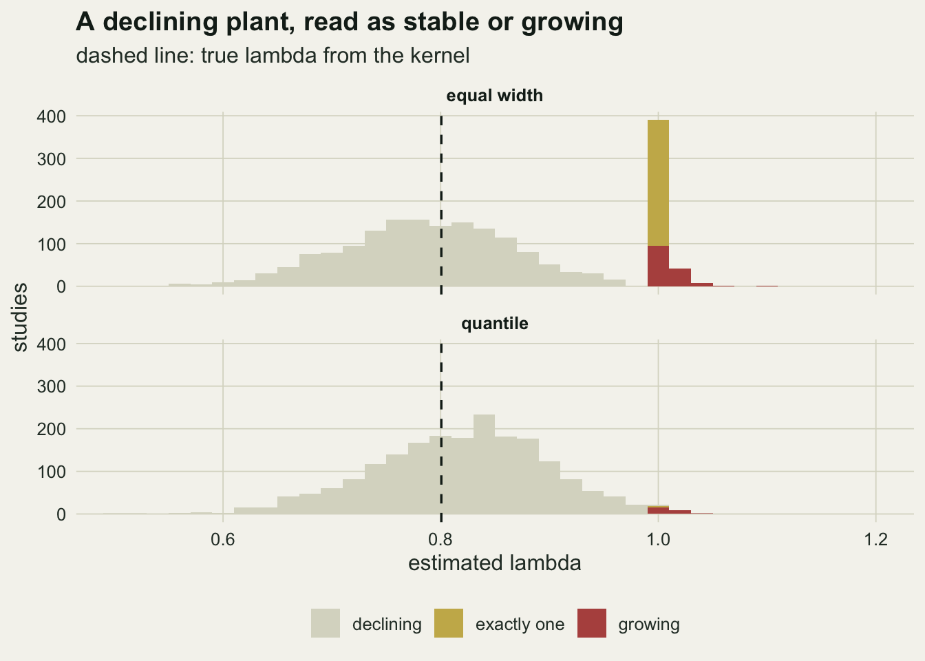
A class with one plant in it
The spike at exactly one has a closed-form cause. The dominant eigenvalue of a non-negative matrix is at least as large as every entry on its diagonal. A size class that starts with a single plant, which survives and stays in the same class, gets a stasis entry of exactly one, and from then on no amount of mortality elsewhere can bring lambda below one: the matrix says that plant lives forever. Whether lambda stops at one or goes above it depends on whether anything that leaves the class can come back. If nothing can (the plant produced no recruits, or its recruits never grow back into its class), the class is a loop of its own and lambda is exactly one unless the rest of the matrix grows. Only when recruits leave the class and some plant later grows back into it does the class lift lambda above one. Equal-width classes produce singleton classes in the upper tail as a matter of course.
The other half of the mechanism is the sign of the bias. The dominant eigenvalue is a convex function of the diagonal entries of a non-negative matrix (Cohen 1981), so stasis entries that are unbiased but noisy, as a proportion out of a handful of plants is, would push lambda up on average if the rest of the column were held fixed. It is not held fixed, since stasis and growth share the same plants, and the off-diagonal entries enter differently with no general sign, so the size and sign of the whole bias are measured below rather than derived.
m_e120   <- pool[["120 equal width 20"]]
no_dec   <- m_e120["lambda", ] >= 1 - tol_one
diag_hit <- m_e120["d_max", ] >= 1 - tol_one
share_diag <- mean(diag_hit[no_dec])
p_diag_e  <- mean(diag_hit)
p_diag_q  <- mean(pool[["120 quantile 20"]]["d_max", ] >= 1 - tol_one)
typ_e120 <- m_e120["d_type", ]
is_one   <- abs(m_e120["lambda", ] - 1) <= tol_one
is_grow  <- m_e120["lambda", ] > 1 + tol_one
n_one    <- sum(is_one)
n_one_by <- vapply(0:3, function(t) sum(is_one & typ_e120 == t), 0)
n_grow   <- sum(is_grow)
n_grow_cyc <- sum(is_grow & typ_e120 == 3)
cyc_all_grow <- all(m_e120["lambda", typ_e120 == 3] > 1 + tol_one)

set.seed(3104)
m_obs <- run_cell(n_cell, 120, 20, "equal width, observed range")
obs_grow <- mean(m_obs["lambda", ] > 1 + tol_one)
obs_one  <- mean(abs(m_obs["lambda", ] - 1) <= tol_one)
top_obs <- replicate(n_cell, {
  z_s <- draw_sizes(120)
  brk <- class_breaks(z_s, 20, "equal width, observed range")
  sum(z_s >= brk[20])
})
top_alone <- mean(top_obs == 1)
In the equal-width studies of 120 plants and 20 classes, 20.8 per cent of matrices have some diagonal entry of one or more, against 1.2 per cent under quantile boundaries. Of the equal-width studies that fail to show the decline, 94 per cent carry such an entry, which by the eigenvalue bound is enough on its own to explain the verdict. Whether that entry gives exactly one or more than one is decided by the path back. Of the 295 studies at exactly one, 98 have a class that nothing leaves (its plants stayed and produced no recruits), 186 have a class whose recruits leave it with no path in the matrix leading back, none has a class with a diagonal entry of one or more on a cycle, and 11 reach one without any diagonal entry of one. Of the 148 growing studies, 129 have a class with a diagonal entry of one or more on a cycle, recruits out and a plant back in, and every study with such a cycle grows.
The fixed axis from 0 to 12 might look like the cause, since it reaches far past the largest plant. It is not. Cutting the equal-width classes between the smallest and the largest plant in the sample instead, which is what most people would do with real data, makes it worse at twenty classes: 9.8 per cent of studies grow and 24.3 per cent sit at exactly one. The top class then always contains the largest plant in the sample, and in 54 per cent of samples it contains nothing else.
No class count to recommend
The same grid gives the error curve in the class count, which is the question Vandermeer and Moloney posed as a balance: fine classes reduce distribution error, and each one also holds fewer plants, so its transitions carry more sampling error. For lambda in this design the balance turns out to have only one side, and the limit with unlimited plants shows why. With every plant followed, each column of the matrix is the kernel averaged over the stable distribution inside the class, and that collapsed matrix can be computed directly for any set of boundaries.
best_k <- function(nn, ru) {
  s <- cells[cells$n == nn & cells$rule == ru, ]
  vapply(seq_len(n_run), function(r) {
    s_r <- s[s$run == r, ]
    s_r$k[which.min(s_r$rmse)]
  }, 0)
}
bk_e400 <- best_k(400, "equal width")
bk_q400 <- best_k(400, "quantile")
bk_e120 <- best_k(120, "equal width")
bk_q120 <- best_k(120, "quantile")

eq_rows <- grid_tab[grid_tab$rule == "equal width", ]
qu_rows <- grid_tab[grid_tab$rule == "quantile", ]
q_wins_rmse <- all(qu_rows$rmse < eq_rows$rmse)
q_wins_bias <- all(abs(qu_rows$bias) < abs(eq_rows$bias))
q400_rng <- range(qu_rows$rmse[qu_rows$n == 400])
e400_rng <- range(eq_rows$rmse[eq_rows$n == 400])
ratio_e400 <- e400$rmse / cell_of(400, "equal width", 4)$rmse
ratio_q400 <- q400$rmse / cell_of(400, "quantile", 4)$rmse
e120_3 <- cell_of(120, "equal width", 3)
e120_2 <- cell_of(120, "equal width", 2)

collapse_kernel <- function(brk) {
  cls  <- findInterval(kern_400$mesh, brk, all.inside = TRUE)
  memb <- outer(cls, seq_len(length(brk) - 1), "==") * 1
  wt   <- memb * w_stab
  cw   <- pmax(colSums(wt), 1e-300)
  p_c  <- sweep(t(memb) %*% kern_400$P %*% wt, 2, cw, "/")
  f_c  <- sweep(t(memb) %*% kern_400$F %*% wt, 2, cw, "/")
  lam_and_elas(p_c, f_c)
}
stab_breaks <- function(k) c(z_lo, sapply(seq_len(k - 1) / k, stab_q), z_hi)
lim_tab <- data.frame(k = k_grid,
  lam_eq = vapply(k_grid, function(kk) collapse_kernel(seq(z_lo, z_hi, length.out = kk + 1))[["lambda"]], 0),
  lam_qu = vapply(k_grid, function(kk) collapse_kernel(stab_breaks(kk))[["lambda"]], 0),
  ef_qu  = vapply(k_grid, function(kk) collapse_kernel(stab_breaks(kk))[["e_fec"]], 0))
lim_gap <- max(abs(c(lim_tab$lam_eq, lim_tab$lam_qu) - lam_true))
Across all 14 collapsed matrices, both rules and every class count from 2 to 20, the dominant eigenvalue equals the kernel’s to within floating-point rounding. That is exact aggregation, not luck: summing the stable distribution within classes gives a right eigenvector of the collapsed matrix with the same eigenvalue, whatever the boundaries. The plants in these studies are drawn from the stable distribution, so lambda carries no distribution error at all here; every bit of its error, and every difference between class counts, is sampling error. The elasticity, which also needs the left eigenvector, is not protected in the same way, and a later section shows it.
Quantile boundaries give the smaller root mean square error in every one of the 14 cells, and the smaller absolute bias in every one. At 400 plants the quantile error stays between 0.0352 and 0.0389 over the whole range of class counts, while the equal-width error runs from 0.0448 to 0.0829; twenty classes cost 1.26 times the error of four under equal width and 1.11 times under quantiles.
The class count that minimises the error is not a transferable answer. Under equal width the best count in each of the five runs was 4, 4, 4, 4, 4 at 120 plants and 2, 2, 2, 2, 2 at 400, so the optimum moved with the sample size, and a two-class matrix of a perennial plant is not a model anyone would publish. Under quantiles the best count was 2, 2, 4, 2, 2 at 120 plants and wandered over 4, 6, 2, 8, 3 at 400, where the curve is so flat that run-to-run noise decides the minimum. With no distribution error to trade against, nothing pulls the minimum towards fine classes, and where it lands is set by sampling noise and by where the boundaries happen to fall. The equal-width curve is not even smooth in k. Three classes put the top boundary at 8, and the top class then expects 0.9 of 120 plants: 14.7 per cent of studies at 120 plants fail to show the decline. Two classes put it at 6, the top class expects 11.8 plants, and 1.7 per cent fail. Where the fixed grid happens to fall against the tail of the size distribution decides the result, which is the opposite of what a neutral rule is supposed to do.
grid_tab$panel <- factor(sprintf("%d plants", grid_tab$n),
                         levels = sprintf("%d plants", n_grid))
p_rmse <- ggplot(grid_tab, aes(k, rmse, colour = rule)) +
  geom_line(linewidth = 0.9) +
  geom_point(size = 2) +
  facet_wrap(~ panel) +
  scale_x_log10(breaks = k_grid) +
  scale_colour_manual(values = rule_cols, name = NULL) +
  labs(x = NULL, y = "RMSE of lambda",
       title = "Quantile boundaries win at every class count") +
  theme_datasheet() +
  theme(legend.position = "none")
p_fail <- ggplot(grid_tab, aes(k, no_decline, colour = rule)) +
  geom_line(linewidth = 0.9) +
  geom_point(size = 2) +
  facet_wrap(~ panel) +
  scale_x_log10(breaks = k_grid) +
  scale_colour_manual(values = rule_cols, name = NULL) +
  labs(x = "number of size classes (log scale)",
       y = "share with lambda of one or more") +
  theme_datasheet() +
  theme(legend.position = "bottom")
(p_rmse / p_fail) + plot_annotation(theme = theme_datasheet())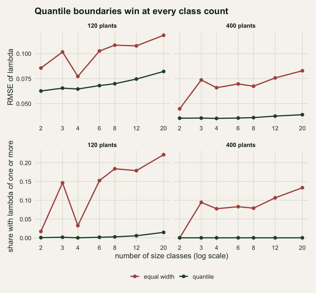
The bias shrinks with sample size
A tempting reading of the last two sections is that the equal-width bias is structural and survives any amount of data. That is false, and the check is cheap: hold the class count at twenty and raise the sample to 1500 and 4000 plants, with the same 2000 studies per cell.
n_big <- c(1500, 4000)
set.seed(7707)
big <- lapply(rules, function(ru) lapply(n_big, function(nn) run_cell(n_cell, nn, 20, ru)))
bias_tab <- rbind(
  grid_tab[grid_tab$k == 20, c("n", "rule", "bias", "bias_se")],
  do.call(rbind, lapply(seq_along(rules), function(i) {
    do.call(rbind, lapply(seq_along(n_big), function(j) {
      lam_v <- big[[i]][[j]]["lambda", ]
      data.frame(n = n_big[j], rule = rules[i], bias = mean(lam_v) - lam_true,
                 bias_se = sd(lam_v) / sqrt(n_cell))
    }))
  })))
bias_of <- function(ru, nn) bias_tab$bias[bias_tab$rule == ru & bias_tab$n == nn]
b_e <- vapply(c(120, 400, n_big), function(nn) bias_of("equal width", nn), 0)
b_q <- vapply(c(120, 400, n_big), function(nn) bias_of("quantile", nn), 0)
fall_e <- b_e[1] / b_e[4]
fall_q <- b_q[1] / b_q[4]
ratio_by_n <- b_e / b_q
bias_falls_e <- b_e[4] < b_e[1]
z_q_big <- b_q[3:4] / bias_tab$bias_se[bias_tab$rule == "quantile" &
                                         bias_tab$n %in% n_big]
Under equal width the bias at twenty classes goes +0.0332, +0.0259, +0.0191, +0.0127 at 120, 400, 1500 and 4000 plants; under quantiles it goes +0.0178, +0.0050, +0.0013, +0.0005. The Monte Carlo standard error of each value is at most 0.0025. The equal-width bias falls by a factor of 2.6 from the smallest sample to the largest. The quantile bias falls faster: at 120 and 400 plants the equal-width bias is 1.9 and 5.2 times the quantile one, and by 1500 and 4000 plants the quantile bias is 3.2 and 2.0 standard errors from zero, so a ratio of the two biases carries too much Monte Carlo error to quote.
Where the two curves are heading was computed in the previous section: with unlimited plants the collapsed matrix returns the true lambda under either rule. So the whole of the bias measured here is small-sample bias in a non-linear function of estimated entries, it goes away with enough plants under either rule, and what the boundary rule decides is how many plants “enough” is. Under equal width the upper classes hold a fixed small share of the sample however large the sample gets, so they reach an adequate count much later than any class a quantile rule cuts.
ggplot(bias_tab, aes(n, bias, colour = rule)) +
  geom_hline(yintercept = 0, colour = te_ink, linewidth = 0.4) +
  geom_errorbar(aes(ymin = bias - 2 * bias_se, ymax = bias + 2 * bias_se),
                width = 0.04, linewidth = 0.6) +
  geom_line(linewidth = 0.9) +
  geom_point(size = 2.4) +
  scale_x_log10(breaks = c(120, 400, 1500, 4000)) +
  scale_colour_manual(values = rule_cols, name = NULL) +
  labs(x = "plants followed for one year (log scale)",
       y = "mean estimate minus true lambda",
       title = "The bias shrinks under both rules",
       subtitle = "twenty classes; bars: two Monte Carlo standard errors") +
  theme_datasheet() +
  theme(legend.position = "bottom")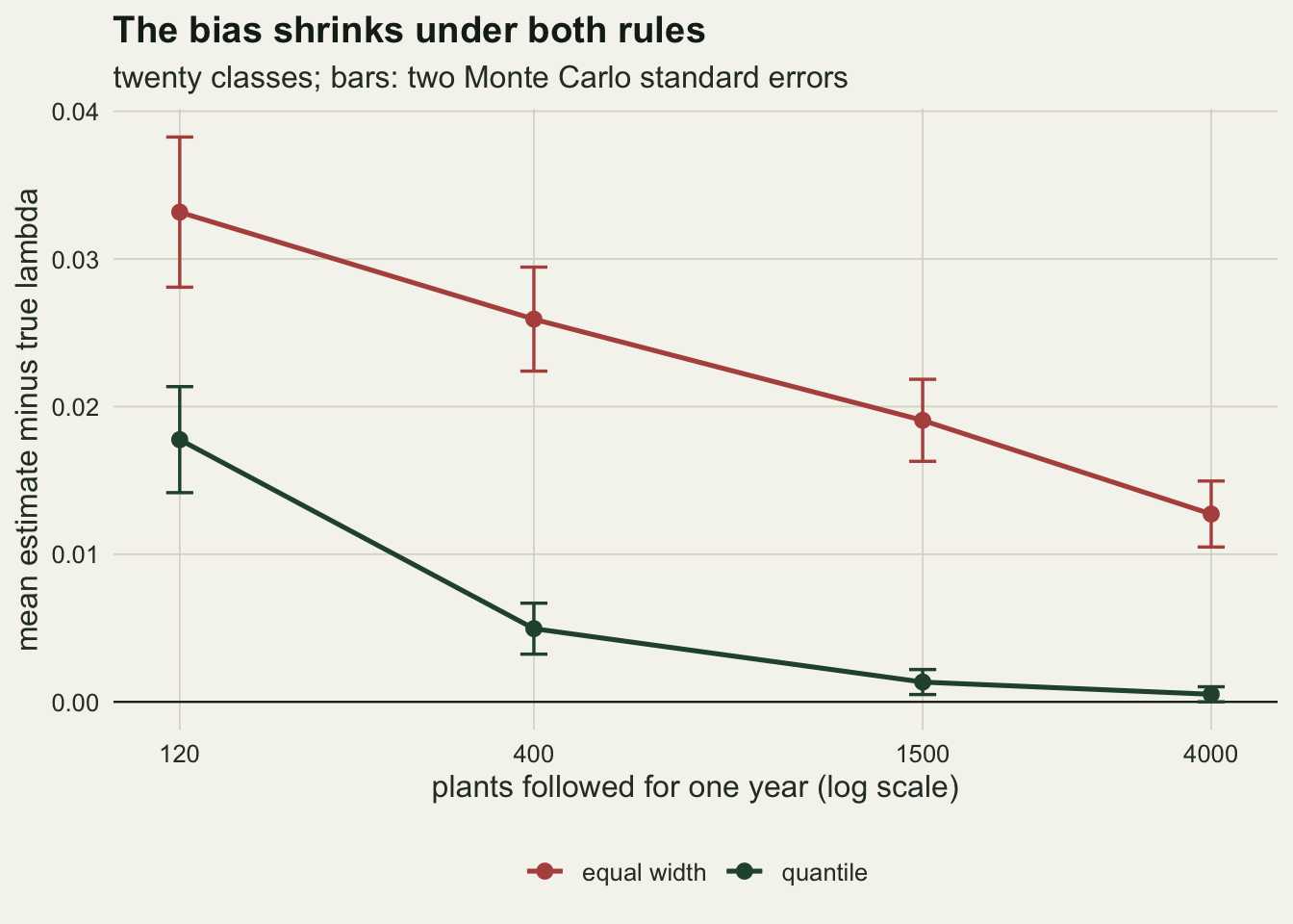
Elasticity pulls the other way
Comparative studies use elasticities more than lambda, and Salguero-Gomez and Plotkin (2010) found that collapsing matrices to fewer classes raised the stasis and fecundity elasticities. The grid above also stored the summed elasticity of lambda to the fecundity entries, computed on the occupied classes of each matrix, and the kernel gives its true value.
ef_e400 <- vapply(k_grid, function(kk) cell_of(400, "equal width", kk)$e_fec, 0)
ef_q400 <- vapply(k_grid, function(kk) cell_of(400, "quantile", kk)$e_fec, 0)
ef_q120_20 <- q120$e_fec
ef_ratio_k2 <- ef_q400[1] / efec_true
ef_lim_2  <- lim_tab$ef_qu[lim_tab$k == 2]
ef_lim_20 <- lim_tab$ef_qu[lim_tab$k == 20]
n_na_total <- sum(grid_tab$e_na)
n_total    <- n_cell * nrow(grid_tab)
The true fecundity elasticity is 0.0765. At 400 plants the quantile rule estimates it at 0.1591 with two classes, 0.1099 with four and 0.0768 with twenty; two classes overstate it by a factor of 2.1. Equal width gives 0.1171 at four classes and 0.0699 at twenty. Coarse classes let a recruit reach adult size in one step, which shortens the life cycle and gives reproduction more weight than it has. This is distribution error, and the collapsed matrices confirm it: with unlimited plants and quantile classes the fecundity elasticity is 0.1584 at two classes and 0.0797 at twenty, so almost all of the two-class overstatement survives any sample size. It pulls towards many classes, the opposite of the pull on lambda. Under quantile boundaries at 400 plants, twenty classes get both quantities close to the truth, with a lambda bias of +0.0050, although part of the elasticity’s closeness is cancellation: its unlimited-sample value at twenty classes is 0.0797, above the truth, and small-sample bias pulls the estimate back down near the truth; at 120 plants the fecundity elasticity at twenty quantile classes is 0.0701, a little under the kernel value, and the lambda bias is +0.0178. The elasticity could not be computed in 27 of the 56000 matrices, which are left out of these means.
ggplot(grid_tab, aes(k, e_fec, colour = rule)) +
  geom_hline(yintercept = efec_true, linetype = "dashed", colour = te_ink,
             linewidth = 0.6) +
  geom_line(linewidth = 0.9) +
  geom_point(size = 2) +
  facet_wrap(~ panel) +
  scale_x_log10(breaks = k_grid) +
  scale_colour_manual(values = rule_cols, name = NULL) +
  labs(x = "number of size classes (log scale)",
       y = "elasticity of lambda to fecundity",
       title = "Few classes inflate the fecundity elasticity",
       subtitle = "dashed line: the value from the 400-bin kernel") +
  theme_datasheet() +
  theme(legend.position = "bottom")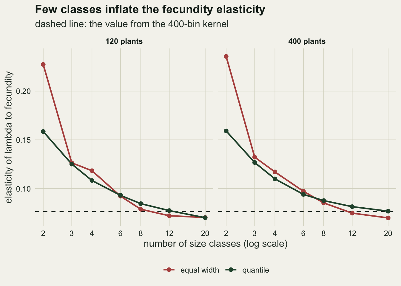
Two checks a reviewer will ask for
Every plant in the kernel above reproduces at a Poisson rate. Real fecundity is rarer and clumpier: most individuals produce nothing in a given year and a few produce many. The first check keeps the mean fecundity at every size exactly as before, so the kernel and its lambda do not change, but lets only a quarter of plants breed, each breeder drawing its recruits from a geometric distribution with the mean scaled up to match. The second check answers the demographer who wants named stages: a fixed stage boundary at size 3, with the classes shared out between the two stages in proportion to the plants in each and cut at quantiles inside each stage.
set.seed(5512)
zi_e  <- run_cell(n_cell, 120, 20, "equal width", fec_type = "zinb")
zi_q  <- run_cell(n_cell, 120, 20, "quantile", fec_type = "zinb")
stg_q <- run_cell(n_cell, 120, 20, "staged quantile")
verdicts <- function(m) {
  lam_v <- m["lambda", ]
  c(grow = mean(lam_v > 1 + tol_one), one = mean(abs(lam_v - 1) <= tol_one),
    bias = mean(lam_v) - lam_true, rmse = sqrt(mean((lam_v - lam_true)^2)))
}
v_zi_e <- verdicts(zi_e)
v_zi_q <- verdicts(zi_q)
v_stg  <- verdicts(stg_q)
zi_fail_e <- v_zi_e[["grow"]] + v_zi_e[["one"]]
With rare, clumped fecundity at twenty classes and 120 plants, 2.8 per cent of equal-width studies grow and 18.1 per cent sit at exactly one, against 7.4 and 14.8 per cent with Poisson fecundity. Studies move from growing to exactly one, because a lone plant in a top class now usually produces no recruits and its class closes on itself; the share that fails to show the decline is 20.9 per cent against 22.1, and the root mean square error is 0.1197 against 0.1184. Under quantiles the rates are 1.6 and 0.3 per cent, against 1.2 and 0.2. The guess that clumped fecundity makes the verdict worse is not what this kernel shows, and the reason is in the elasticity: reproduction carries only 8 per cent of the elasticity of lambda here, so the noise that decides the verdict is in stasis and growth, not in recruits. A shorter-lived plant, whose lambda leans on fecundity, would need its own check.
Quantile classes inside two named stages give 1.4 per cent growing and 0.1 per cent at exactly one, with a bias of +0.0103 against +0.0178 for quantiles over the whole axis. Named stages cost nothing here, so the recommendation that survives is quantile boundaries inside each stage the biology names, not quantiles in place of stages.
What to report
Report the boundary rule as part of the model, next to the number of classes, and report the number of individuals that started in each class. A class that started with one or two individuals is visible in that table at once, and the eigenvalue bound says what it can do: a stasis entry of one sets a floor of one under lambda, whatever the rest of the matrix says.
Cut boundaries where the individuals are. Quantiles of this year’s sizes, inside any stages the biology fixes, take one line of R. They gave a smaller error than equal width in every cell of the grid, and no cell let more than 1.5 per cent of quantile studies miss the decline, against up to 22.1 per cent under equal width. They are not Moloney’s algorithm, which balances the two errors class by class and is not tested here; they are the cheap rule that stops a class from being cut where nobody lives.
Do not report a class count as the answer. The best count moved between runs, and under equal width at 400 plants it was a two-class matrix. When the class count matters for the question, as it does for elasticities, show lambda and the elasticities at two or three class counts under the same boundary rule, which costs a loop.
State the verdict with an interval that includes this source of error. A bootstrap that resamples individuals and re-cuts the classes inside every resample carries the boundary rule into the interval’s width (not tested here); a bootstrap of vital rates within fixed classes does not. Neither removes the bias, since both are centred on the biased estimate.
Honest limits
The kernel is one plant: slow, declining by 20 per cent a year, with lambda carried mostly by stasis and growth. The wrong-verdict rates depend on how far lambda sits from one. A population declining by five per cent a year sits closer to the line, so the same spread of estimates would cross it more often under either rule; that case is not simulated here, and the rates quoted are for this kernel, to be read as the order of the effect and not as a constant. The exactly-one verdicts depend much less on that distance, because a singleton class that closes on itself puts a floor of one under lambda whatever the rest of the matrix says.
Each study follows its plants for one year. A multi-year study pools transitions and fills the sparse classes faster, although the upper classes under equal width stay a fixed small share of the pool. Plants were drawn from the stable size distribution, and that choice removed distribution error from lambda by construction, as the collapsed matrices showed. A population far from its stable structure, which a declining one may well be, has a different size structure, different empty classes and a distribution error on lambda as well, so the balance Vandermeer described comes back for lambda too; this post measured only the sampling side of it.
Moloney’s algorithm itself is not run here, and nor are any of the methods Picard, Ouedraogo and Bar-Hen compared. The comparison is between the rule most people use and the one-line rule that fixes most of it, and it says nothing about how much further a full optimisation of the boundaries would go.
The elasticity result covers one summed elasticity, to fecundity. Salguero-Gomez and Plotkin (2010) also report shifts in progression and retrogression elasticities, which are not measured here, and element-level elasticities cannot be compared across class counts at all.
The integral projection model avoids the whole choice by estimating smooth regressions that borrow strength across sizes, as in building an integral projection model, but it moves the decision into the form of those regressions rather than removing it; nothing here compares the two.
References
Vandermeer J 1978 Oecologia 32(1):79-84 (10.1007/BF00344691)
Moloney KA 1986 Oecologia 69(2):176-180 (10.1007/BF00377618)
Picard N, Ouedraogo D-Y, Bar-Hen A 2010 Ecological Modelling 221(19):2270-2279 (10.1016/j.ecolmodel.2010.06.010)
Salguero-Gomez R, Plotkin JB 2010 American Naturalist 176(6):710-722 (10.1086/657044)
Cohen JE 1981 Proceedings of the American Mathematical Society 81(4):657 (10.1090/S0002-9939-1981-0601750-2)