library(readxl)     # reads .xlsx and .xls files
library(openxlsx)   # used here only to build the example workbook
library(ggplot2)

te_paper  <- "#f5f4ee"
te_ink    <- "#16241d"
te_body   <- "#2c3a31"
te_forest <- "#275139"
te_rust   <- "#b5534e"
te_gold   <- "#c9b458"
te_line   <- "#dad9ca"

theme_datasheet <- function() {
  theme_minimal(base_size = 12) +
    theme(plot.background  = element_rect(fill = te_paper, colour = NA),
          panel.background = element_rect(fill = te_paper, colour = NA),
          panel.grid.major = element_line(colour = te_line, linewidth = 0.3),
          panel.grid.minor = element_blank(),
          text             = element_text(colour = te_body),
          axis.text        = element_text(colour = te_body),
          strip.text       = element_text(colour = te_ink, face = "bold"))
}Reading Excel field sheets into R
R
data import
readxl
missing data
data cleaning
ecology tutorial
Read an Excel field sheet into R with readxl: why a count typed as text after row 1000 becomes NA, and why a date column with text arrives as serial numbers.
A winter of wetland bird counts, typed by volunteers into one Excel workbook: a row for each species on each count, with the date, the species and the number of birds. By the end of March the sheet has 1500 rows. Two habits of the counters are in it. Faced with a big flock late in the season, some of them typed an estimate such as c. 80 instead of a number. And where a count’s date was lost, somebody typed not recorded in the date column.
Reading field data into R reads a CSV with read.csv(), which looks at every value in a column before it decides the column’s type, so one n/a turns the whole column into text and the first sum() fails. An .xlsx file read with the readxl package behaves differently. read_excel() decides each column’s type from the first 1000 rows only, and a text entry further down that is not a number does not change the type: it becomes NA, with a warning that is easy never to see. Dates have their own problem. Excel stores a date as a number of days, and when that number reaches R as text you need the right starting day to turn it back. Dates and times in ecological data parses dates written as text with a format string; the serial numbers here need an origin instead.
The short answer. Tell read_excel() what each column is with col_types, and list your missing-value codes in na. Read a column that mixes numbers and notes as text, and turn it into numbers yourself, so that every entry that is not a plain number is counted rather than dropped. A date serial that arrives as text converts with as.Date(as.numeric(x), origin = "1899-12-30"), and a check on the weekday of your count dates catches an origin that is off by a day or two.
The workbook below is simulated and built in the code, and every seed is in the code.
A workbook to read
The counts are made on Sundays, one of the 26 Sundays from October to the end of March for each row, and the rows are in date order, as a sheet typed up during the season would be. Counts start at 1, because a species with no birds gets no row.
set.seed(2410)
n_rows <- 1500
sundays <- seq(as.Date("2023-10-01"), by = "week", length.out = 26)
stopifnot(all(as.POSIXlt(sundays)$wday == 0))   # 0 is Sunday

visit_true <- sort(sample(sundays, n_rows, replace = TRUE))
species    <- sample(c("teal", "wigeon", "mallard", "lapwing", "golden plover"),
                     n_rows, replace = TRUE)
count_pool <- 1 + rnbinom(n_rows, mu = 19, size = 1.5)
Sixty rows after row 1000 hold the text entries. The function below writes the sheet with openxlsx: the counts as numbers, then the chosen cells overwritten with text, then five dates overwritten with not recorded. Your own data would already be a file, data/counts.xlsx, and the first line of your script would be the read_excel() call in the next section.
n_text   <- 60
text_row <- sort(1000 + sample(n_rows - 1000, n_text))   # data rows 1001 to 1500
no_date  <- sort(sample(1000, 5))                         # lost dates, all in the first 1000 rows

build_sheet <- function(count, text_row, text_entry, file_name) {
  wb <- createWorkbook()
  addWorksheet(wb, "counts")
  writeData(wb, "counts", data.frame(visit = visit_true, species = species, count = count))
  for (k in seq_along(text_row)) {       # + 1 because row 1 of the sheet is the header
    writeData(wb, "counts", text_entry[k], startCol = 3, startRow = text_row[k] + 1, colNames = FALSE)
  }
  for (k in no_date) {
    writeData(wb, "counts", "not recorded", startCol = 1, startRow = k + 1, colNames = FALSE)
  }
  path <- file.path(tempdir(), file_name)
  saveWorkbook(wb, path, overwrite = TRUE)
  path
}
In the first sheet the estimates are the big flocks. The 60 largest counts go to the 60 text rows, and each is written the way a counter writes a flock that cannot be counted bird by bird: rounded to ten, with c. in front. sheet_value holds the number each counter meant.
big_first <- order(count_pool, decreasing = TRUE)
count_big <- integer(n_rows)
count_big[text_row]  <- sample(count_pool[big_first[1:n_text]])       # sample() shuffles
count_big[-text_row] <- sample(count_pool[big_first[-(1:n_text)]])
flock_value <- pmax(10, round(count_big[text_row], -1))

sheet_value <- count_big
sheet_value[text_row] <- flock_value
path_flocks <- build_sheet(count_big, text_row, paste("c.", flock_value), "counts.xlsx")
head(paste("c.", flock_value))
[1] "c. 100" "c. 70" "c. 70" "c. 60" "c. 60" "c. 60" The estimates run from c. 50 to c. 120, and every plain count left on the sheet is at most 54.
read_excel() guesses from the first 1000 rows
A plain call, as the first line of a script would make it. The warnings are collected into a vector here so that the page stays readable. At the console R reports warnings once the call returns, but more than ten arrive as a single line telling you to run warnings(), which then lists only the first 50. A rendered report with warnings turned off shows none of them.
read_quietly <- function(...) {
  caught <- character(0)
  out <- withCallingHandlers(read_excel(...), warning = function(w) {
    caught <<- c(caught, conditionMessage(w))
    invokeRestart("muffleWarning")
  })
  list(data = out, warnings = caught)
}

default_read <- read_quietly(path_flocks)
counts <- default_read$data
str(counts)
tibble [1,500 × 3] (S3: tbl_df/tbl/data.frame)
$ visit : chr [1:1500] "45200" "45200" "45200" "45200" ...
$ species: chr [1:1500] "teal" "lapwing" "golden plover" "teal" ...
$ count : num [1:1500] 25 4 15 16 13 4 26 11 12 6 ...length(default_read$warnings)[1] 60head(default_read$warnings, 2)[1] "Expecting numeric in C1002 / R1002C3: got 'c. 100'"
[2] "Expecting numeric in C1003 / R1003C3: got 'c. 70'" stopifnot(packageVersion("readxl") >= "1.4.0",
identical(formals(read_excel)$guess_max, quote(min(1000, n_max))),
identical(formals(read_excel)$n_max, Inf),
is.numeric(counts$count), sum(is.na(counts$count)) == n_text,
length(default_read$warnings) == n_text,
all(is.na(counts$count[text_row])), !anyNA(counts$count[-text_row]),
getOption("nwarnings") == 50) # warnings() keeps at most 50The count column came back as numbers, and 60 of its 1500 values are NA: exactly the 60 cells that held an estimate. readxl reads the first guess_max rows to decide a column’s type, and the default is min(1000, n_max), so 1000 rows for a whole sheet (this is readxl 1.5.0.1 here, and the source of readxl 1.5.0 has the same default). The readxl article on cell and column types (Wickham and Bryan 2026) describes the rest of the rule: a column with text among its guessed rows becomes text, the type of last resort. All 1000 of those rows held plain numbers, so the column became numeric. Each later cell that could not be a number was set to NA, and each one produced a warning naming the cell, 60 warnings in all.
plot_rows <- data.frame(row = seq_len(n_rows), value = sheet_value,
                        status = ifelse(is.na(counts$count), "typed as text: read as NA", "number: read"))

ggplot(plot_rows, aes(row, value)) +
  annotate("rect", xmin = 0.5, xmax = 1000.5, ymin = 1, ymax = 400, fill = te_line, alpha = 0.6) +
  annotate("text", x = 500, y = 330, label = "guess window: rows 1 to 1000",
           colour = te_ink, size = 3.8) +
  geom_point(aes(colour = status, size = status), alpha = 0.75) +
  scale_colour_manual(values = c("number: read" = te_forest, "typed as text: read as NA" = te_rust)) +
  scale_size_manual(values = c("number: read" = 0.9, "typed as text: read as NA" = 1.9)) +
  scale_y_log10(limits = c(1, 400)) +
  labs(x = "row of the sheet", y = "birds counted (log scale)", colour = NULL, size = NULL) +
  theme_datasheet() +
  theme(legend.position = "top")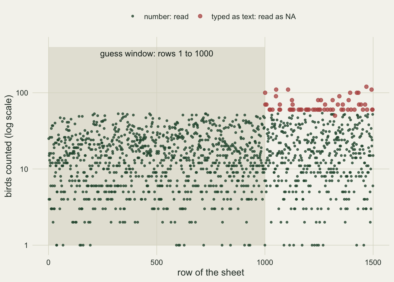
The NA then travels. mean(count, na.rm = TRUE) skips it without a word, and so does every summary that drops missing values (Missing values in summaries measures what that does to a total).
mean_sheet <- mean(sheet_value)
mean_read  <- mean(counts$count, na.rm = TRUE)
round(c(on_the_sheet = mean_sheet, as_read = mean_read,
        change_per_cent = 100 * (mean_read / mean_sheet - 1)), 2)
on_the_sheet as_read change_per_cent
19.96 17.86 -10.52 mean_text <- mean(sheet_value[text_row])
stopifnot(isTRUE(all.equal(mean_read,
mean_sheet - n_text / (n_rows - n_text) * (mean_text - mean_sheet))))The counters meant a mean of 19.96 birds per row. The column as read gives 17.86, 10.5 per cent less, because the rows that were lost are the biggest flocks of the winter. The size of the drop is arithmetic, not a property of readxl. Take k values with mean m_text away from n values with mean m, and the mean of the rest is m - k * (m_text - m) / (n - k). Here k is 60, n is 1500 and the lost estimates average 70.33 birds, which gives the 17.86 above; the last line of the chunk checks it.
Which cells became NA sets the direction
A smaller mean is not a rule. The column loses whichever rows were typed as text, and the mean moves towards the rows that are left. In a second sheet, the same 60 rows hold the smallest counts instead, typed with a question mark by a counter who was unsure of the number (2?).
small_first <- order(count_pool)
count_small <- integer(n_rows)
count_small[text_row]  <- sample(count_pool[small_first[1:n_text]])
count_small[-text_row] <- sample(count_pool[small_first[-(1:n_text)]])
path_unsure <- build_sheet(count_small, text_row, paste0(count_small[text_row], "?"), "counts_unsure.xlsx")

unsure_read <- read_quietly(path_unsure)
mean_sheet_unsure <- mean(count_small)
mean_read_unsure  <- mean(unsure_read$data$count, na.rm = TRUE)
round(c(on_the_sheet = mean_sheet_unsure, as_read = mean_read_unsure,
        change_per_cent = 100 * (mean_read_unsure / mean_sheet_unsure - 1)), 2)
on_the_sheet as_read change_per_cent
19.93 20.70 3.85 stopifnot(sum(is.na(unsure_read$data$count)) == n_text, length(unsure_read$warnings) == n_text,
mean_read_unsure > mean_sheet_unsure, mean_read < mean_sheet)Again 60 values are NA and 60 warnings were raised, and this time the mean goes up, from 19.93 to 20.70. The same reading step moves the mean one way on one sheet and the other way on the next, and the size of the move depends on how many cells were text and how far their values sit from the rest. The lost values cannot be recovered from the data frame afterwards: an NA marks where a value was, not what it was, and only the warnings kept the text.
means_long <- data.frame(
  sheet  = rep(c("big flocks typed as 'c. 60'", "small counts typed as '2?'"), times = 2),
  source = rep(c("numbers the counters wrote", "column as read by read_excel()"), each = 2),
  value  = c(mean_sheet, mean_sheet_unsure, mean_read, mean_read_unsure))

ggplot(means_long, aes(value, sheet)) +
  geom_line(aes(group = sheet), colour = te_line, linewidth = 1.4) +
  geom_point(aes(colour = source), size = 3.6) +
  scale_colour_manual(values = c("numbers the counters wrote" = te_forest,
                                 "column as read by read_excel()" = te_rust)) +
  labs(x = "mean birds per row", y = NULL, colour = NULL) +
  theme_datasheet() +
  theme(legend.position = "top")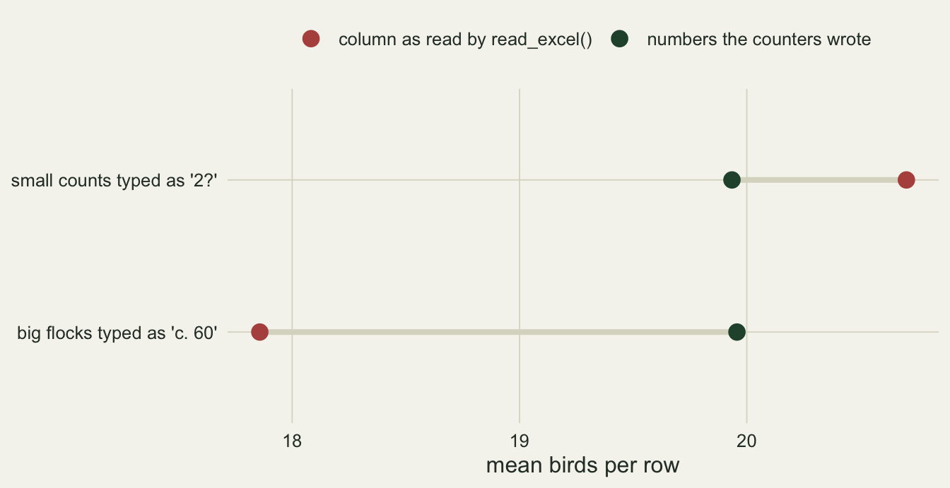
One text cell early changes the whole column
Now move a single estimate from the second half of the flock sheet into the first 1000 rows, to row 500.
early_row <- text_row
early_row[1] <- 500
count_early <- count_big
count_early[c(500, text_row[1])] <- count_big[c(text_row[1], 500)]
path_early <- build_sheet(count_early, early_row, paste("c.", flock_value), "counts_early.xlsx")

early_read <- read_quietly(path_early)
class(early_read$data$count)
[1] "character"length(early_read$warnings)[1] 0sum_attempt <- try(sum(early_read$data$count), silent = TRUE)
conditionMessage(attr(sum_attempt, "condition"))[1] "invalid 'type' (character) of argument"stopifnot(is.character(early_read$data$count), length(early_read$warnings) == 0,
inherits(try(sum(early_read$data$count), silent = TRUE), "try-error"))One text cell inside the guess window is enough: the column comes back as text, with 0 warnings, and sum() fails exactly as it does after read.csv(). This is the better outcome. The failure is loud and it happens at the first calculation, while the column that came back as numbers in the previous section ran every calculation without an error.
Tell read_excel() what the columns are
Two arguments deal with the guess. guess_max can be raised so that the guess looks at every row; a value larger than the sheet, such as 100000, is enough (Inf also works, with a warning that it has been lowered to a large finite number).
whole_guess <- read_quietly(path_flocks, guess_max = 100000)
class(whole_guess$data$count)
[1] "character"length(whole_guess$warnings)[1] 0inf_guess <- read_quietly(path_flocks, guess_max = Inf)
stopifnot(is.character(whole_guess$data$count), length(whole_guess$warnings) == 0,
is.character(inf_guess$data$count), length(inf_guess$warnings) == 1,
grepl("guess_max", inf_guess$warnings[1]))With every row in the guess, the flock column comes back as text. That is safe, but it is still a guess. col_types states the types outright, one per column, and na lists the entries that mean missing. The date column is declared as a date and the count column as text, so that each estimate can be dealt with on purpose:
typed_read <- read_quietly(path_flocks, col_types = c("date", "text", "text"),
                           na = c("", "not recorded"))
typed <- typed_read$data
length(typed_read$warnings)
[1] 0typed$is_estimate <- grepl("^c\\.", typed$count)
typed$birds <- as.numeric(sub("^c\\.\\s*", "", typed$count))
c(estimates = sum(typed$is_estimate), missing_counts = sum(is.na(typed$birds))) estimates missing_counts
60 0 round(mean(typed$birds), 2)[1] 19.96stopifnot(length(typed_read$warnings) == 0, sum(typed$is_estimate) == n_text,
!anyNA(typed$birds), isTRUE(all.equal(mean(typed$birds), mean_sheet)),
sum(is.na(typed$visit)) == length(no_date))No warnings, 60 estimates found and kept as numbers, 0 missing counts, and the mean is the 19.96 birds per row that the counters meant. The is_estimate column keeps the information the c. carried, so an analysis can still leave the estimates out or give them their own error, but that is now a decision in the script rather than a side effect of the reader. If a pattern like ^c\. is new to you, Text and regular expressions in R covers it.
Dates that arrive as serial numbers
Back to the plain read_excel() call. Look at its first column.
class(counts$visit)[1] "character"head(counts$visit, 4)[1] "45200" "45200" "45200" "45200"stopifnot(is.character(counts$visit), sum(counts$visit == "not recorded") == length(no_date),
all(grepl("^[0-9]{5}$", counts$visit[-no_date])))The visit dates came back as text: apart from the five not recorded cells, every entry is a five-digit number such as 45200. Those five cells sit inside the first 1000 rows, so the guess for the column was text, and a date cell in a text column arrives as the number Excel stores behind it: the date serial, a count of days. With na = c("", "not recorded") in the call, as in the typed read above, the same column arrives as a date-time:
class(typed$visit)[1] "POSIXct" "POSIXt" attr(typed$visit, "tzone")[1] "UTC"visit_read <- as.Date(typed$visit)
stopifnot(inherits(typed$visit, "POSIXct"), identical(attr(typed$visit, "tzone"), "UTC"),
all(visit_read[-no_date] == visit_true[-no_date]))readxl returns dates as date-times in UTC, and as.Date() turns them into plain dates; all 1495 of them match the true visit dates. When a file has already been read and you have the serials as text, the conversion needs an origin, the day R counts the serials from. For dates from March 1900 on in Excel’s default 1900 date system, that day is 30 December 1899 (why not 1 January 1900 is explained below):
serial <- as.numeric(counts$visit[-no_date])
right_origin <- as.Date(serial, origin = "1899-12-30")
jan_origin   <- as.Date(serial, origin = "1900-01-01")
no_origin    <- as.Date(serial)
truth        <- visit_true[-no_date]
new_year      <- sum(format(jan_origin, "%Y") != format(truth, "%Y"))
out_of_season <- sum(jan_origin < as.Date("2023-10-01") | jan_origin > as.Date("2024-03-31"))

c(days_off_1899_12_30 = unique(as.numeric(right_origin - truth)),
  days_off_1900_01_01 = unique(as.numeric(jan_origin - truth)))
days_off_1899_12_30 days_off_1900_01_01
0 2 range(format(no_origin, "%Y"))[1] "2093" "2094"stopifnot(all(right_origin == truth), all(jan_origin - truth == 2),
getRversion() >= "4.3.0", as.Date(0) == as.Date("1970-01-01"),
getDateOrigin(path_flocks) == "1900-01-01",
all(convertToDate(serial, origin = getDateOrigin(path_flocks)) == truth),
as.Date(61, origin = "1899-12-30") == as.Date("1900-03-01"),
as.Date(40729, origin = "1899-12-30") == as.Date("2011-07-05"),
as.Date(39267, origin = "1904-01-01") == as.Date("2011-07-05"),
as.numeric(as.Date("1904-01-01") - as.Date("1899-12-30")) == 1462,
new_year > 0, new_year == sum(format(truth, "%m-%d") == "12-31"), out_of_season == 0,
all(truth - 1462 == as.Date(paste0(as.numeric(format(truth, "%Y")) - 4, format(truth, "-%m-%d"))) - 1))The origin 1899-12-30 gives every date exactly. The origin that looks right, 1 January 1900, puts every date 2 days late. And as.Date() with no origin at all uses 1 January 1970 (R has done so since version 4.3.0; older versions stop with an error), which moves this winter to the years 2093 to 2094. That one is easy to spot. The two-day error is not: every date is plausible, inside the field season, and wrong. The 50 rows dated 31 December have even moved into the next year.
The two days come from Excel itself. Excel counts 1 January 1900 as day 1, not day 0, and it treats 1900 as a leap year, so it has a 29 February 1900 that never happened (serial 60). Microsoft documents the extra leap day as a choice made for compatibility with Lotus 1-2-3 and kept ever since. From 1 March 1900 on, each serial is two more than the number of days since 1 January 1900. openxlsx (4.2.9 here; the current source does the same) has a pair of functions for this: getDateOrigin() reports the workbook’s date system as "1900-01-01", and convertToDate() subtracts the two days when given that origin. Passing the output of getDateOrigin() straight to as.Date() gives the two-day error again.
The quickest check on converted dates is the one the design gives you for free. These counts were all made on Sundays:
day_names <- c("Sun", "Mon", "Tue", "Wed", "Thu", "Fri", "Sat")
weekday_of <- function(d) factor(day_names[as.POSIXlt(d)$wday + 1], levels = day_names)
rbind(origin_1899_12_30 = table(weekday_of(right_origin)),
      origin_1900_01_01 = table(weekday_of(jan_origin)),
      no_origin         = table(weekday_of(no_origin)))
Sun Mon Tue Wed Thu Fri Sat
origin_1899_12_30 1495 0 0 0 0 0 0
origin_1900_01_01 0 0 1495 0 0 0 0
no_origin 0 0 0 0 0 1495 0weekday_long <- data.frame(
origin = factor(rep(c("origin 1899-12-30", "origin 1900-01-01", "no origin (1970-01-01)"),
each = length(serial)),
levels = c("origin 1899-12-30", "origin 1900-01-01", "no origin (1970-01-01)")),
weekday = c(weekday_of(right_origin), weekday_of(jan_origin), weekday_of(no_origin)))
weekday_long$correct <- weekday_long$origin == "origin 1899-12-30"
ggplot(weekday_long, aes(weekday, fill = correct)) +
geom_bar(width = 0.7) +
scale_x_discrete(drop = FALSE) +
scale_fill_manual(values = c("TRUE" = te_forest, "FALSE" = te_rust), guide = "none") +
facet_wrap(~ origin) +
labs(x = NULL, y = "visits") +
theme_datasheet() +
theme(axis.text.x = element_text(size = 8))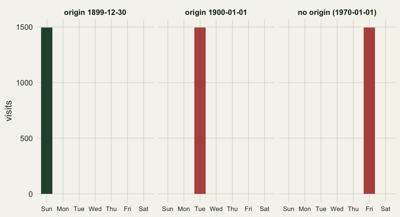
A table of weekdays takes one line and turns a silent two-day shift into a column of Tuesdays. The same check works for any sampling design with a fixed day. A range check against the field season is no substitute: it catches the 2090s at once, but after the two-day shift 0 of the 1495 dates fall outside October to March. Without a fixed weekday, compare a few converted dates with the paper sheets or a field diary.
The origin 1899-12-30 has two limits of its own. It is exact only for serials from 61 on, dates from 1 March 1900, which covers any modern field sheet. And it holds only for the 1900 date system. Workbooks set to the 1904 date system, the old default in Excel for Mac, count days from 1 January 1904, and a serial from such a file needs origin = "1904-01-01". Using 1899-12-30 instead would put every date 1462 days early, four years and one day, which is the gap Microsoft gives between the two systems. Its worked example, 5 July 2011, is serial 40729 in the 1900 system and 39267 in the 1904 system, and each converts to the right day with the matching origin. getDateOrigin() tells you which system a file uses.
What to check in your own data
Run str() after every read_excel() call, as after read.csv(), and read the type of each column against what it should be. A count column that is chr has text in its first 1000 rows; a count column that is num may still have lost text entries further down, which only the warnings or a count of NA values will show.
Count the NA values in each column straight after reading, with colSums(is.na(x)), and compare them with the blank cells you expect. Every extra one is a cell the reader could not turn into the type it guessed.
The lasting fix is on the sheet. Broman and Woo (2018) ask for one thing in each cell, with notes in a column of their own, and for every cell to be filled, with one agreed code for missing values. On this sheet that means a plain number in the count column with a yes in an estimate column beside it, and one missing-value code in the date column, the same code everywhere, with the reason in the notes.
For a sheet you will read more than once, write col_types and na into the call. Read columns that mix numbers with notes as "text", and parse them with a line of code that you can check.
Convert date serials with origin = "1899-12-30", or with convertToDate() and getDateOrigin(), and then check the dates against the design: the weekday if the survey had one, otherwise a few dates against the paper sheets. A range check catches the 1970 origin, not a two-day shift.
Honest limits
The workbooks here were written by openxlsx, not by Excel, and they have one sheet, a header row and no merged cells, colours or formulas. A field workbook typed in Excel can carry all of those, and readxl’s treatment of formatted cells (a number stored as text, a date typed in a cell formatted as text) is not tested here. The 1904 date system is described from its definition, not demonstrated: openxlsx writes 1900-system workbooks. The sizes of the two mean shifts belong to these two constructed sheets; they show that the direction depends on which cells were text, and say nothing about how large the shift is in real count data.
References
Broman KW, Woo KH 2018 The American Statistician 72(1):2-10 (10.1080/00031305.2017.1375989)
Wickham H, Bryan J 2026 readxl 1.5.0 documentation: Cell and column types (https://readxl.tidyverse.org/articles/cell-and-column-types.html)
Microsoft 2026 Excel troubleshooting: Excel incorrectly assumes that the year 1900 is a leap year (https://learn.microsoft.com/en-us/troubleshoot/microsoft-365-apps/excel/wrongly-assumes-1900-is-leap-year)
Microsoft 2024 Excel help: Date systems in Excel (https://support.microsoft.com/en-us/office/date-systems-in-excel-e7fe7167-48a9-4b96-bb53-5612a800b487)