library(ggplot2)
library(patchwork)

te_paper  <- "#f5f4ee"
te_ink    <- "#16241d"
te_body   <- "#2c3a31"
te_forest <- "#275139"
te_rust   <- "#b5534e"
te_gold   <- "#c9b458"
te_line   <- "#dad9ca"

theme_datasheet <- function() {
  theme_minimal(base_size = 12) +
    theme(plot.background  = element_rect(fill = te_paper, colour = NA),
          panel.background = element_rect(fill = te_paper, colour = NA),
          panel.grid.major = element_line(colour = te_line, linewidth = 0.3),
          panel.grid.minor = element_blank(),
          text             = element_text(colour = te_body),
          plot.title       = element_text(colour = te_ink, face = "bold"),
          plot.subtitle    = element_text(colour = te_body),
          axis.text        = element_text(colour = te_body),
          strip.text       = element_text(colour = te_ink, face = "bold"))
}Pielou’s evenness under unequal sampling effort
R
diversity
evenness
rarefaction
biodiversity
simulation
ecology tutorial
Pielou’s J ranks two communities by sampling effort, not evenness, when effort differs. Simulate it in R, rarefy to a common n, and see what coverage adds.
A restoration team compares the aquatic invertebrates of a restored pond with those of an old reference pond nearby. The reference pond has been kick-sampled for years and its pooled sample holds a thousand individuals; the restored pond was sampled once, in a wet week, and the sample holds a hundred. The report gives richness and Shannon for both, then adds Pielou’s evenness, J, the Shannon index divided by the log of the number of species seen, “to separate richness from evenness”. The restored pond comes out the more even of the two, and the sentence in the discussion writes itself: the new community is not yet dominated by a few colonists.
That sentence can be produced by the sampling alone. J is a ratio of two sample statistics, and both of them fall short of their true values in a small sample, by different amounts. This is not a new observation. Soetaert and Heip showed in 1990 that diversity indices, Hill’s numbers among them, depend on sample size, in samples from a high-diversity deep-sea environment, and Bulinski set out in 2007 how evenness behaves as a function of sample size along a palaeoenvironmental gradient. This post is a demonstration of that known result, not a claim to it. What it measures is narrower and practical: how often J ranks two communities the wrong way when their effort differs, how that depends on the true difference, what happens when one community is sampled twice, which repairs work, and where the bias changes sign.
Computing diversity indices in R with vegan lists Pielou’s evenness (shannon / log(richness)) among its next steps and does not test it. When not to use the Shannon index computes the same ratio once, on complete communities, and has a section showing that Shannon itself is biased downward in small samples; it names a distortion of evenness without giving its direction. Estimating diversity with Hill numbers shows that plug-in diversity is biased low and that the bias shrinks as the order q rises, and its chao1() and shannon_CS() are the parts of one of the repairs that fails below.
The closest relative is Checking a beta diversity analysis. The beta post shows a ratio of diversities inflating as effort falls, and shows that equal effort does not make two differently structured regions comparable; Pielou’s J does both inside a single sample. Rarefying to the smaller sample removes the effort difference almost completely, as more effort does within one region of the beta post, and what it leaves behind is the structural limit the beta post found, in a milder form: at equal n, the richer of two equally even communities reads as the more even.
Two communities, one sampled ten times harder
Every community below has a lognormal species abundance distribution. For the ranking comparison the shapes are deterministic: the relative abundances of S species are the lognormal quantiles at evenly spaced probabilities, and the log standard deviation is tuned by root finding until the true J hits a target. That removes the luck of one random community from the comparison and leaves only sampling noise. A sample of n individuals is a multinomial draw from the true proportions.
The helpers compute every index from a species by sample matrix of counts in one pass. J is the plug-in Shannon index over the log of the observed richness. Three repairs change the index and keep the sample: plug-in Shannon over the log of Chao1, the Chao and Shen coverage-adjusted Shannon over the log of Chao1 (the same two estimators as the Hill number post), and the ratio of inverse Simpson to exponential Shannon, D2/D1, which contains no richness at all. Two classic alternatives from the evenness literature are carried along: Heip’s index, (exp(H) - 1)/(S - 1), and Smith and Wilson’s Evar, one minus 2/pi times the arctangent of the variance of log abundances across the species present. Two repairs change the effort and keep J: rarefying the larger sample to the size of the smaller, and rarefying the sample with the higher estimated coverage down to the coverage of the other, using the Chao and Jost coverage estimator and their formula for the expected coverage of a subsample.
det_sad <- function(S, sd_log) {
  a_s <- qlnorm(ppoints(S), 0, sd_log)
  a_s / sum(a_s)
}
true_J  <- function(p) -sum(p * log(p)) / log(length(p))
tune_sd <- function(S, target)
  uniroot(function(s) true_J(det_sad(S, s)) - target, c(0.02, 5))$root

ev_idx <- function(X) {
  n_i  <- colSums(X)
  pres <- X > 0
  s_ob <- colSums(pres)
  P    <- sweep(X, 2, n_i, "/")
  H    <- -colSums(ifelse(pres, P * log(P), 0))
  D2   <- 1 / colSums(P^2)
  f1   <- colSums(X == 1)
  f2   <- colSums(X == 2)
  chao <- s_ob + (n_i - 1) / n_i * f1 * (f1 - 1) / (2 * (f2 + 1))
  c_gt <- 1 - ifelse(f1 == n_i, n_i - 1, f1) / n_i
  PA   <- sweep(P, 2, c_gt, "*")
  NM   <- matrix(n_i, nrow(X), ncol(X), byrow = TRUE)
  H_cs <- -colSums(ifelse(pres, PA * log(PA) / (1 - (1 - PA)^NM), 0))
  LX   <- ifelse(pres, log(X), 0)
  m_lx <- matrix(colSums(LX) / s_ob, nrow(X), ncol(X), byrow = TRUE)
  v_lx <- colSums(ifelse(pres, (LX - m_lx)^2, 0)) / s_ob
  cbind(J = H / log(s_ob), J_chao = H / log(chao), J_cs = H_cs / log(chao),
        hill21 = D2 / exp(H), heip = (exp(H) - 1) / (s_ob - 1),
        evar = 1 - 2 / pi * atan(v_lx), S = s_ob, H = H)
}

# one random subsample of m individuals from each column, without replacement
rarefy_cols <- function(X, m) {
  m_left <- rep_len(m, ncol(X))
  n_left <- colSums(X)
  out    <- matrix(0L, nrow(X), ncol(X))
  for (i in seq_len(nrow(X) - 1)) {
    k_i      <- rhyper(ncol(X), X[i, ], n_left - X[i, ], m_left)
    out[i, ] <- k_i
    n_left   <- n_left - X[i, ]
    m_left   <- m_left - k_i
  }
  out[nrow(X), ] <- m_left
  out
}

cov_hat <- function(x) {
  n <- sum(x); f1 <- sum(x == 1); f2 <- sum(x == 2)
  if (f1 == 0) return(1)
  if (f2 == 0) return(1 - (f1 / n) * ((n - 1) * (f1 - 1) / ((n - 1) * (f1 - 1) + 2)))
  1 - (f1 / n) * ((n - 1) * f1 / ((n - 1) * f1 + 2 * f2))
}
cov_at_m <- function(x, m) {
  n <- sum(x); x <- x[x > 0]
  1 - sum((x / n) * exp(lchoose(n - x, m) - lchoose(n - 1, m)))
}
m_for_cov <- function(x, target) {
  n <- sum(x); lo <- 1; hi <- n - 1
  if (cov_at_m(x, hi) < target) return(n)
  while (hi - lo > 1) {
    mid <- (lo + hi) %/% 2
    if (cov_at_m(x, mid) >= target) hi <- mid else lo <- mid
  }
  hi
}
# the sample with the higher coverage is brought down to the other's coverage
cov_sizes <- function(XA, XB) {
  c_a <- apply(XA, 2, cov_hat)
  c_b <- apply(XB, 2, cov_hat)
  m_a <- vapply(seq_len(ncol(XA)), function(j)
    if (c_a[j] > c_b[j]) m_for_cov(XA[, j], c_b[j]) else sum(XA[, j]), 0)
  m_b <- vapply(seq_len(ncol(XB)), function(j)
    if (c_b[j] > c_a[j]) m_for_cov(XB[, j], c_a[j]) else sum(XB[, j]), 0)
  list(a = m_a, b = m_b)
}
# mean of J, Heip and Evar over n_avg independent subsamples
avg_rare <- function(X, m, n_avg) {
  if (all(m == colSums(X))) return(ev_idx(X)[, c("J", "heip", "evar")])
  Reduce(`+`, lapply(seq_len(n_avg), function(k)
    ev_idx(rarefy_cols(X, m))[, c("J", "heip", "evar")])) / n_avg
}
Community A has 60 species and a true J of 0.80. Community B has the same 60 species and a true J lower by a fixed contrast. The design grid was fixed before anything ran: four contrasts from 0.03 to 0.14, and four effort pairs, written as individuals in A / individuals in B. The denominator for every rate in this section is the pair of samples: one sample from A and one from B, and the rate is the share of pairs in which A, the truly more even community, gets the higher value.
S_rank    <- 60
J_high    <- 0.80
contrasts <- c(0.03, 0.05, 0.08, 0.14)
eff_pairs <- list(c(1000, 100), c(100, 1000), c(150, 600), c(300, 300))
n_pair    <- 2000
n_avg     <- 20
mc_se_max <- sqrt(0.25 / n_pair)

sd_high <- tune_sd(S_rank, J_high)
p_high  <- det_sad(S_rank, sd_high)
set.seed(3727)
rank_tab <- NULL
for (cc in contrasts) {
  p_low <- det_sad(S_rank, tune_sd(S_rank, J_high - cc))
  tr_a  <- ev_idx(matrix(p_high * 1e9))
  tr_b  <- ev_idx(matrix(p_low * 1e9))
  for (ep in eff_pairs) {
    XA  <- rmultinom(n_pair, ep[1], p_high)
    XB  <- rmultinom(n_pair, ep[2], p_low)
    m_c <- min(ep)
    XA1 <- if (ep[1] > m_c) rarefy_cols(XA, m_c) else XA
    XB1 <- if (ep[2] > m_c) rarefy_cols(XB, m_c) else XB
    rA  <- avg_rare(XA, rep(m_c, n_pair), n_avg)
    rB  <- avg_rare(XB, rep(m_c, n_pair), n_avg)
    m_cv <- cov_sizes(XA, XB)
    cA  <- avg_rare(XA, m_cv$a, n_avg)
    cB  <- avg_rare(XB, m_cv$b, n_avg)
    iA  <- ev_idx(XA)
    iB  <- ev_idx(XB)
    rank_tab <- rbind(rank_tab, data.frame(
      contrast = cc, pair = paste(ep, collapse = " / "),
      naive    = mean(iA[, "J"] > iB[, "J"]),
      rare_one = mean(ev_idx(XA1)[, "J"] > ev_idx(XB1)[, "J"]),
      rare_avg = mean(rA[, "J"] > rB[, "J"]),
      cov_avg  = mean(cA[, "J"] > cB[, "J"]),
      chao     = mean(iA[, "J_chao"] > iB[, "J_chao"]),
      cs       = mean(iA[, "J_cs"] > iB[, "J_cs"]),
      hill21   = mean(iA[, "hill21"] > iB[, "hill21"]),
      heip     = mean(iA[, "heip"] > iB[, "heip"]),
      evar     = mean(iA[, "evar"] > iB[, "evar"]),
      heip_r   = mean(rA[, "heip"] > rB[, "heip"]),
      evar_r   = mean(rA[, "evar"] > rB[, "evar"]),
      same_order = all(c(tr_a[, "hill21"] > tr_b[, "hill21"],
                         tr_a[, "heip"] > tr_b[, "heip"],
                         tr_a[, "evar"] > tr_b[, "evar"]))))
  }
}
rk <- function(cc, pr, col) rank_tab[rank_tab$contrast == cc & rank_tab$pair == pr, col]
all_same_order <- all(rank_tab$same_order)

# how many observed species are singletons or doubletons in a 100-individual sample of B
set.seed(3732)
X_thin    <- rmultinom(n_pair, 100, det_sad(S_rank, tune_sd(S_rank, J_high - 0.05)))
low_share <- mean(colSums(X_thin == 1 | X_thin == 2) / colSums(X_thin > 0))

# the pond case at 100 individuals: expected J of A and B, and the Chao1 version
set.seed(3733)
p_b05  <- det_sad(S_rank, tune_sd(S_rank, J_high - 0.05))
n_big  <- 20000
iA100  <- ev_idx(rmultinom(n_big, 100, p_high))
iB100  <- ev_idx(rmultinom(n_big, 100, p_b05))
iA1000 <- ev_idx(rmultinom(n_pair, 1000, p_high))
EJA100 <- mean(iA100[, "J"])
EJB100 <- mean(iB100[, "J"])
fresh_100 <- mean(iA100[seq_len(n_pair), "J"] > iB100[seq_len(n_pair), "J"])
known_a   <- mean(EJA100 > iB100[, "J"])
sd_J_B    <- sd(iB100[, "J"])
sd_chao_B <- sd(iB100[, "J_chao"])
chao_A1000 <- mean(iA1000[, "J_chao"])
chao_B100  <- mean(iB100[, "J_chao"])
The replication was fixed at 2000 sample pairs per cell before the simulation ran, so the Monte Carlo standard error of any rate below is at most 0.011. The tuned log standard deviation for A is 1.377.
Take the pond case: the truly more even community A sampled at 1000 individuals, B at 100, and a true contrast of 0.05. Naive J calls A the more even in 0.101 of pairs. It is wrong in 0.899 of pairs, and wrong in a consistent direction: the thin sample reads as the more even. Rarefying A to 100 individuals with one random subsample, which is what vegan::rrarefy() does, puts the rate at 0.808, and averaging J over 20 independent subsamples raises it to 0.862.
Swap the efforts, so that the truly more even community is the thin sample, and naive J is right in 1.000 of pairs. That is not the index working. The bias points the same way as the truth and flatters the community that happened to be sampled lightly. At equal effort, 300 individuals each, naive J is right in 0.934 of pairs: that is the ceiling for this contrast at that effort. The averaged rarefied rate at 1000 / 100, 0.862, sits below it because the comparison now happens at 100 individuals. At n = 100 the expected J is 0.871 for A and 0.843 for B, so the expected contrast shrinks from 0.05 to 0.028, and B’s single sample of 100 is noisy. Two fresh samples of 100 each rank the pair correctly in 0.819 of pairs, and knowing A’s expected J at 100 exactly, against one sample of 100 from B, would only lift the rate to 0.885. The averaged rarefied rate lies between those two.
The headline depends on the contrast, which is why the figure shows the whole axis rather than one number. At the smallest contrast, 0.03, naive J is right in 0.037 of pairs; at 0.08, in 0.278; at 0.14, in 0.763. A large true difference survives the bias most of the time, and a small one is reversed nearly always.
Coverage rarefaction does not beat size rarefaction on this comparison. Averaged over 20 subsamples it is right in 0.781 of pairs at the contrast of 0.05, against 0.862 for size rarefaction, and at equal effort it falls to 0.901 because it discards individuals from whichever sample has the higher estimated coverage even when the two sizes already match. The two communities here share S = 60, which is the case size rarefaction is built for; the last section of the post shows the case where coverage earns its place.
at_1000 <- rank_tab[rank_tab$pair == "1000 / 100", ]
long_rank <- function(cols, labs) {
  do.call(rbind, lapply(seq_along(cols), function(k)
    data.frame(contrast = at_1000$contrast, share = at_1000[[cols[k]]],
               estimator = labs[k])))
}
lab_eff <- c("naive J", "rarefied, one subsample", "rarefied, mean of 20",
             "equal coverage, mean of 20")
lab_idx <- c("naive J", "H / ln Chao1", "Chao-Shen H / ln Chao1", "D2 / D1",
             "Heip", "Evar")
d_eff <- long_rank(c("naive", "rare_one", "rare_avg", "cov_avg"), lab_eff)
d_idx <- long_rank(c("naive", "chao", "cs", "hill21", "heip", "evar"), lab_idx)
d_eff$estimator <- factor(d_eff$estimator, levels = lab_eff)
d_idx$estimator <- factor(d_idx$estimator, levels = lab_idx)

rank_panel <- function(d_p, cols, ttl) {
  ggplot(d_p, aes(contrast, share, colour = estimator, shape = estimator)) +
    geom_hline(yintercept = 0.5, linetype = "dotted", colour = te_body,
               linewidth = 0.4) +
    geom_line(linewidth = 0.8) +
    geom_point(size = 2.2) +
    scale_colour_manual(values = cols, name = NULL) +
    scale_shape_manual(values = c(16, 17, 15, 18, 3, 4)[seq_along(cols)], name = NULL) +
    scale_x_continuous(breaks = contrasts) +
    scale_y_continuous(limits = c(0, 1)) +
    labs(x = "true J of A minus true J of B", y = "share ranked correctly",
         title = ttl) +
    theme_datasheet() +
    guides(colour = guide_legend(ncol = 2), shape = guide_legend(ncol = 2)) +
    theme(legend.position = "bottom")
}
p_eff <- rank_panel(d_eff, c(te_ink, te_gold, te_forest, te_rust),
                    "Change the effort")
p_idx <- rank_panel(d_idx, c(te_ink, "#3f6e8c", "#8a6a4f", "#7d8f86", "#8c5a7a", "#9e9e9e"),
                    "Change the index")
(p_eff | p_idx) +
  plot_annotation(subtitle = "A (true J 0.80) sampled at 1000 individuals, B at 100; 2000 sample pairs per point",
                  theme = theme_datasheet())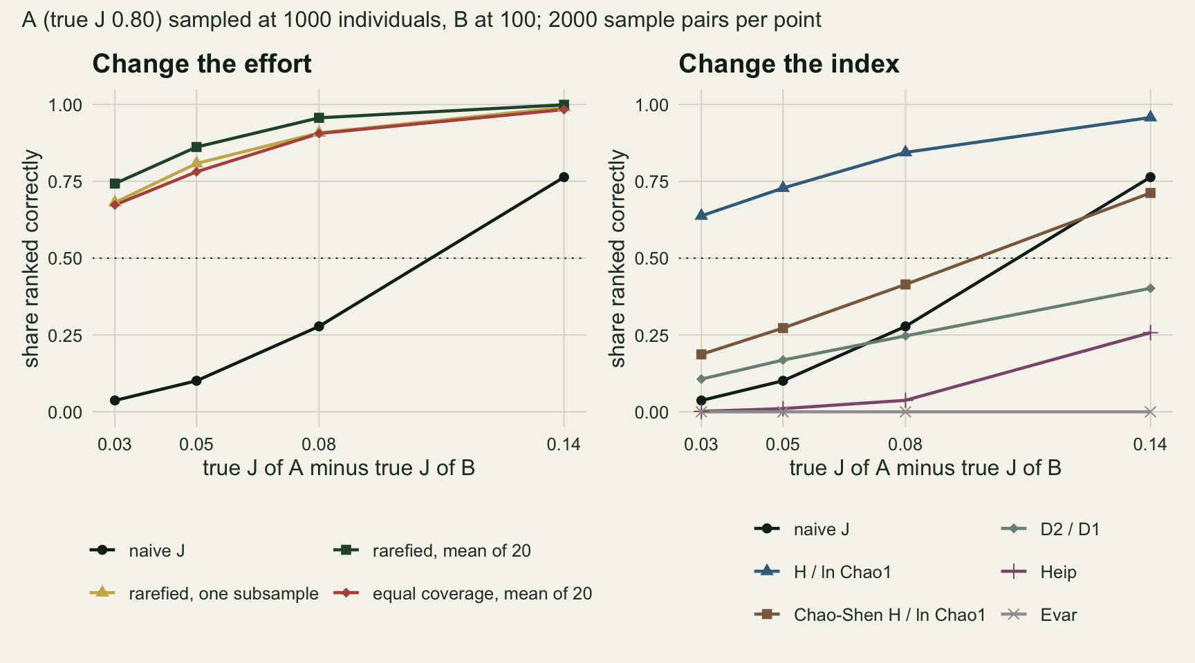
Changing the index instead of the effort
The right panel is the one most readers would reach for first, because it leaves the data alone. None of those repairs matches rarefaction; the Chao1 version comes nearest, 0.080 below one-subsample rarefaction and 0.134 below the averaged version. At the contrast of 0.05 and 1000 / 100, plug-in H over the log of Chao1 is right in 0.728 of pairs, the Chao-Shen version in 0.273, and the richness-free ratio D2/D1 in 0.169. For all three indices, and for Heip and Evar, the true values rank A above B at every contrast (checked in the chunk), so these rates measure the same question as the rates for J.
The Chao1 version does best of the three, and it is not a repair. At these tuned shapes it is close to unbiased for A and far less biased than J for B: at the contrast of 0.05 it averages 0.799 for A at 1000 individuals and 0.767 for B at 100, against true values of 0.80 and 0.75 (plain J averages 0.843 for B at 100). That is because these shapes sit where the shortfalls of H and of Chao1 happen to cancel; the next section shows the same index overcorrecting for more even communities. It still loses to rarefaction because Chao1 from 100 individuals is noisy: the standard deviation of H over the log of Chao1 across B’s samples of 100 is 0.050, against 0.024 for J, 2.0 times as large, and the expected gap between A at 1000 and B at 100 is 0.032 rather than the true 0.05, which is still wider than the 0.028 left to rarefied J, so it is the noise that costs the ranking. The Chao-Shen version corrects the numerator upward, which pushes the thin sample up again. D2/D1 is interesting because it has no richness in it at all and still fails: the ratio of two Hill numbers of different order inherits the q ordering of plug-in bias that the Hill number post shows, where D1 is biased more than D2, so the thin sample’s ratio is inflated.
Heip’s index and Evar do worse than J, not better. Naive Heip is right in 0.011 of pairs and naive Evar in 0.000 at 1000 / 100. Evar is the extreme case. In a sample of 100 individuals from community B at that contrast, 0.619 of the observed species on average are singletons or doubletons, so the variance of the log counts is small and the index reads as very even. After averaged rarefaction to 100 both recover, to 0.838 for Heip and 0.852 for Evar, against 0.862 for rarefied J. At equal effort of 300 each, Evar is right in 0.818 of pairs against 0.934 for J. Neither index is a reason to replace rarefied J in this comparison.
Which way the bias runs
The ranking result has a direction in it: the thin sample reads as more even. That direction is not universal. The grid below uses random lognormal communities rather than tuned ones, three richness levels, five log standard deviations and six sample sizes, with five random communities per cell and 200 samples from each.
S_set  <- c(40, 60, 100)
sd_set <- c(0.5, 1.0, 1.3, 1.5, 2.0)
n_set  <- c(50, 100, 200, 500, 1000, 5000)
n_comm <- 5
n_samp <- 200
set.seed(3728)
eff_tab <- NULL
for (S in S_set) for (sd_l in sd_set) for (k in seq_len(n_comm)) {
  p_k <- rlnorm(S, 0, sd_l)
  p_k <- p_k / sum(p_k)
  H_t <- -sum(p_k * log(p_k))
  for (n in n_set) {
    ii <- ev_idx(rmultinom(n_samp, n, p_k))
    eff_tab <- rbind(eff_tab, data.frame(S = S, sdlog = sd_l, comm = k, n = n,
      J_true = true_J(p_k), J_mean = mean(ii[, "J"]), J_sd = sd(ii[, "J"]),
      J_chao = mean(ii[, "J_chao"]), H_rel = mean(ii[, "H"]) / H_t,
      lnS_rel = mean(log(ii[, "S"])) / log(S)))
  }
}
eff_tab$bias <- eff_tab$J_mean - eff_tab$J_true
med_tab <- aggregate(cbind(J_true, bias, J_chao, H_rel, lnS_rel) ~ S + sdlog + n,
                     eff_tab, median)
md <- function(S, sd_l, n, col) med_tab[med_tab$S == S & med_tab$sdlog == sd_l & med_tab$n == n, col]

# gap between n = 100 and n = 1000, per community, in replicate SDs at n = 100
gap_tab <- do.call(rbind, lapply(split(eff_tab, list(eff_tab$S, eff_tab$sdlog, eff_tab$comm)),
  function(d_g) data.frame(S = d_g$S[1], sdlog = d_g$sdlog[1],
    gap = d_g$J_mean[d_g$n == 100] - d_g$J_mean[d_g$n == 1000],
    gap_sd = (d_g$J_mean[d_g$n == 100] - d_g$J_mean[d_g$n == 1000]) / d_g$J_sd[d_g$n == 100])))
gap_med <- aggregate(cbind(gap, gap_sd) ~ S + sdlog, gap_tab, median)
gm <- function(S, sd_l, col) gap_med[gap_med$S == S & gap_med$sdlog == sd_l, col]

# share of communities whose mean J falls at every step of effort, by log SD
mono_c <- aggregate(J_mean ~ S + sdlog + comm, eff_tab[order(eff_tab$n), ],
                    function(v) all(diff(v) < 0))
mono_sd <- aggregate(J_mean ~ sdlog, mono_c, mean)
ms <- function(sd_l) mono_sd$J_mean[mono_sd$sdlog == sd_l]

# spread of true J among random communities drawn from one lognormal
jt_rng <- aggregate(J_true ~ S + sdlog, eff_tab[eff_tab$n == 50, ], function(v) diff(range(v)))
rng_mid <- median(jt_rng$J_true[jt_rng$sdlog %in% c(1.0, 1.3, 1.5)])
For uneven communities J is biased upward, and the bias shrinks with effort. At S = 100 and a log standard deviation of 1.5, the median true J is 0.823 and the median bias is +0.118 at 50 individuals, +0.087 at 100, +0.024 at 1000 and +0.005 at 5000. The difference between the expected J at 100 and at 1000 individuals is 0.069 there, which is 4.4 standard deviations of J between replicate samples of 100. The effort effect is several times the sampling noise of a single sample.
For very even communities the sign reverses, weakly. At a log standard deviation of 0.5 the true J is 0.971 at S = 40, and the median bias at 100 individuals is -0.022; at S = 100 it is -0.010. The statement “J falls as you sample more” is therefore a statement about uneven communities. The share of communities whose mean J fell at every step of effort was 1.00 at a log standard deviation of 2.0, 1.00 at 1.5, 0.93 at 1.3, 0.40 at 1.0 and 0.00 at 0.5.
The mechanism is the arithmetic of the two parts. At S = 100, log standard deviation 1.5 and 100 individuals, the median sample recovers 0.890 of the true Shannon index but only 0.801 of the true log richness: the missing species are rare, they carry little of H, and each one removes the same amount from the denominator as a common species would. The denominator loses more, so the ratio rises. In the very even community at the same S and n the recovered shares are 0.879 for H and 0.887 for log richness: the missing species are not rare any more, H’s own downward bias dominates, and the ratio falls. The q ordering of plug-in bias in the Hill number post predicts the direction for uneven communities; it does not predict the size, or the point where the sign turns.
This is also where the Chao1 reference shows what it is doing. At S = 100 and 50 individuals, H over the log of Chao1 gives 0.804 for a community whose true J is 0.976, 0.800 for one at 0.876, and 0.797 for one at 0.823. The last row comes near its truth only because the downward bias of H and the downward bias of Chao1 happen to cancel there; read beside the other two rows, the index barely moves while the truth moves a great deal.
med_tab$sd_lab <- factor(sprintf("sdlog %.1f", med_tab$sdlog),
                         levels = sprintf("sdlog %.1f", sd_set))
med_tab$S_lab  <- factor(sprintf("S = %d", med_tab$S), levels = sprintf("S = %d", S_set))
ggplot(med_tab, aes(n, bias, colour = sd_lab)) +
  geom_hline(yintercept = 0, colour = te_body, linewidth = 0.4) +
  geom_line(linewidth = 0.8) +
  geom_point(size = 1.8) +
  facet_wrap(~ S_lab, nrow = 1) +
  scale_x_log10(breaks = n_set) +
  scale_colour_manual(values = c(te_gold, te_forest, "#7d8f86", te_rust, te_ink),
                      name = NULL) +
  labs(x = "individuals in the sample (log scale)", y = "expected J minus true J",
       title = "Thin samples read as more even, unless the community already is",
       subtitle = "median over five random communities per line") +
  theme_datasheet() +
  theme(legend.position = "bottom", axis.text.x = element_text(angle = 45, hjust = 1))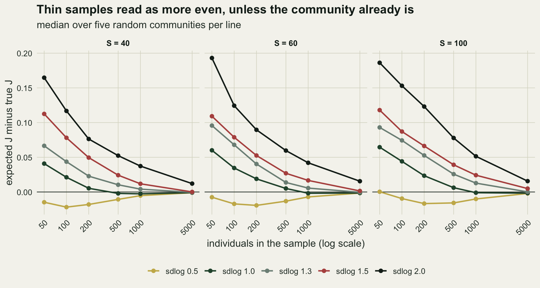
Where the sign turns
To place the turning point, the tuned deterministic shapes are used again, at S = 40 and S = 100, for true J from 0.85 to 0.97 in steps of 0.01, with 2000 samples per point at 100 and at 1000 individuals.
J_sweep <- seq(0.85, 0.97, by = 0.01)
n_sweep <- 2000
set.seed(3729)
cross_tab <- NULL
for (S in c(40, 100)) for (jt in J_sweep) {
  p_s <- det_sad(S, tune_sd(S, jt))
  for (n in c(100, 1000)) {
    ii <- ev_idx(rmultinom(n_sweep, n, p_s))
    cross_tab <- rbind(cross_tab, data.frame(S = S, J_true = jt, n = n,
      bias = mean(ii[, "J"]) - jt, se = sd(ii[, "J"]) / sqrt(n_sweep)))
  }
}
zero_at <- function(y_v, x_v) if (all(y_v < 0) || all(y_v > 0)) NA else approx(y_v, x_v, xout = 0)$y
cross_at <- function(S, n) {
  d_s <- cross_tab[cross_tab$S == S & cross_tab$n == n, ]
  zero_at(d_s$bias, d_s$J_true)
}
gap_at <- function(S) {
  b1 <- cross_tab[cross_tab$S == S & cross_tab$n == 100, "bias"]
  b2 <- cross_tab[cross_tab$S == S & cross_tab$n == 1000, "bias"]
  zero_at(b1 - b2, J_sweep)
}
x40 <- cross_at(40, 100); x100 <- cross_at(100, 100)
g40 <- gap_at(40);        g100 <- gap_at(100)
all_neg_40_1000 <- all(cross_tab$bias[cross_tab$S == 40 & cross_tab$n == 1000] < 0)
x100_1000 <- cross_at(100, 1000)
gap_pos_100 <- all(cross_tab$bias[cross_tab$S == 100 & cross_tab$n == 100] -
                   cross_tab$bias[cross_tab$S == 100 & cross_tab$n == 1000] > 0)
se_max_cross <- max(cross_tab$se)
At 100 individuals the bias crosses zero at a true J of 0.923 for S = 40 and 0.962 for S = 100. The turning point moves with richness, and it moves with effort too: at 1000 individuals the bias at S = 40 is negative across the whole sweep, and at S = 100 it crosses at 0.893. The Monte Carlo standard error of every point is below 0.0005.
For comparing two samples of one community what matters is not the sign of the bias but the sign of the gap, expected J at 100 minus expected J at 1000. At S = 40 that gap crosses zero at a true J of 0.935: below it the thinner sample reads as the more even, above it the thicker one does, by a small amount. At S = 100 the gap stays positive across the whole sweep, up to a true J of 0.97: the bias at 1000 individuals turns negative earlier, at the 0.893 found above, and stays below the bias at 100 individuals, so the thin sample still reads as the more even where both biases are negative.
Is a true difference of 0.05 in J, the pond case above, a realistic difference between two habitats? The effort grid gives one reference: among five random communities drawn from the same lognormal, with log standard deviations of 1.0 to 1.5, the median range of true J is 0.116. Differences of the size used in the ranking comparison arise between communities drawn from one and the same abundance model, so a contrast of 0.05 is not an exotic difference to be looking for.
cross_tab$n_lab <- factor(sprintf("%d individuals", cross_tab$n),
                          levels = c("100 individuals", "1000 individuals"))
cross_tab$S_lab <- factor(sprintf("S = %d", cross_tab$S), levels = c("S = 40", "S = 100"))
v_lines <- data.frame(S_lab = factor(c("S = 40", "S = 100"), levels = c("S = 40", "S = 100")),
                      x_at = c(x40, x100))
ggplot(cross_tab, aes(J_true, bias, colour = n_lab)) +
  geom_hline(yintercept = 0, colour = te_body, linewidth = 0.4) +
  geom_vline(data = v_lines, aes(xintercept = x_at), linetype = "dashed",
             colour = te_rust, linewidth = 0.6) +
  geom_line(linewidth = 0.9) +
  geom_point(size = 1.8) +
  facet_wrap(~ S_lab, nrow = 1) +
  scale_colour_manual(values = c(te_forest, te_gold), name = NULL) +
  scale_x_continuous(breaks = seq(0.85, 0.97, by = 0.03)) +
  labs(x = "true J", y = "expected J minus true J",
       title = "The sign of the bias depends on evenness, richness and effort",
       subtitle = "dashed red: where the bias at 100 individuals crosses zero") +
  theme_datasheet() +
  theme(legend.position = "bottom", panel.spacing = unit(1.5, "lines"))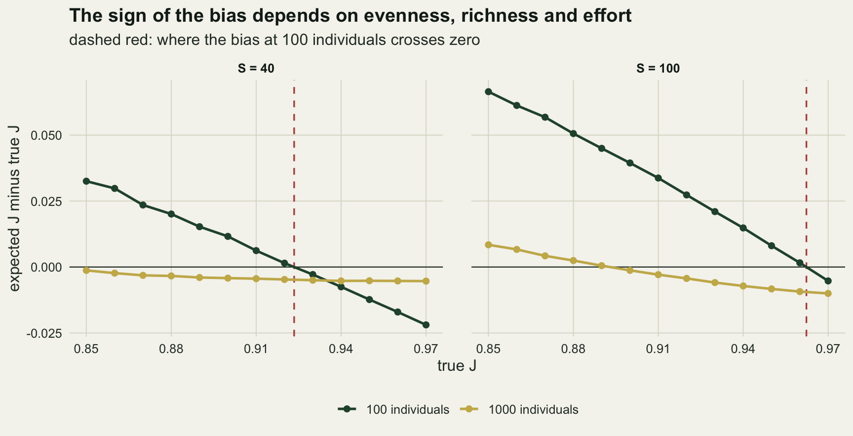
One community, two efforts
The cleanest version of the problem does not need two communities. Take community A, with true J 0.80 and 60 species, and sample it twice, once at 100 individuals and once at 1000. A reader who puts a bootstrap interval on the difference in J and finds that it excludes zero will report that the two samples differ in evenness. The denominator here is the pair of samples from one community, 500 pairs, each with a 95 per cent percentile bootstrap of 200 replicates per sample, resampling individuals within each sample.
boot_J <- function(x, B = 200) ev_idx(rmultinom(B, sum(x), x / sum(x)))[, "J"]
excl0  <- function(d_v) {
  q_v <- quantile(d_v, c(0.025, 0.975))
  unname(q_v[1] > 0 | q_v[2] < 0)
}
n_fd <- 500
set.seed(3730)
fd_mat <- t(replicate(n_fd, {
  x_thin <- rmultinom(1, 100, p_high)[, 1]
  x_full <- rmultinom(1, 1000, p_high)[, 1]
  x_rare <- rarefy_cols(matrix(x_full), 100)[, 1]
  x_cov  <- rarefy_cols(matrix(x_full), m_for_cov(x_full, cov_hat(x_thin)))[, 1]
  b_thin <- boot_J(x_thin)
  j_o <- ev_idx(cbind(x_thin, x_full, x_rare, x_cov))[, "J"]
  c(sig_naive = excl0(b_thin - boot_J(x_full)),
    sig_rare  = excl0(b_thin - boot_J(x_rare)),
    sig_cov   = excl0(b_thin - boot_J(x_cov)),
    d_naive = unname(j_o[1] - j_o[2]), d_rare = unname(j_o[1] - j_o[3]),
    d_cov = unname(j_o[1] - j_o[4]), m_cov = sum(x_cov))
}))
fd_rate <- colMeans(fd_mat[, c("sig_naive", "sig_rare", "sig_cov")])
fd_se   <- sqrt(fd_rate * (1 - fd_rate) / n_fd)
thin_even <- mean(fd_mat[, "d_naive"] > 0)
thin_even_rare <- mean(fd_mat[, "d_rare"] > 0)
m_cov_mean <- mean(fd_mat[, "m_cov"])
The interval excludes zero in 0.696 of pairs (Monte Carlo standard error 0.021), and the thin sample has the higher J in 0.992 of all pairs. The same community, sampled twice, is declared to differ in evenness in more than two pairs out of three.
Rarefy the larger sample to 100 individuals with a single subsample and the rate falls to 0.028 (standard error 0.007); the thin sample now has the higher J in 0.486 of pairs, which is what equal footing looks like. Matching coverage instead gives 0.036: for one community the two standardisations are nearly the same thing, and the coverage-matched subsample averages 104.7 individuals, against the 100 of size rarefaction. This result does not depend on any contrast between communities, which makes it the part of the post least open to argument.
fd_long <- rbind(
  data.frame(d_J = fd_mat[, "d_naive"], cmp = "against the full 1000"),
  data.frame(d_J = fd_mat[, "d_rare"], cmp = "against 1000 rarefied to 100"),
  data.frame(d_J = fd_mat[, "d_cov"], cmp = "against 1000 rarefied to equal coverage"))
fd_long$cmp <- factor(fd_long$cmp, levels = unique(fd_long$cmp))
ggplot(fd_long, aes(d_J)) +
  geom_histogram(binwidth = 0.01, fill = te_forest, colour = te_paper, linewidth = 0.2) +
  geom_vline(xintercept = 0, colour = te_rust, linetype = "dashed", linewidth = 0.6) +
  facet_wrap(~ cmp, ncol = 1) +
  labs(x = "J of the thin sample minus J of the other sample", y = "sample pairs",
       title = "One community, and a difference that is only effort",
       subtitle = "true J 0.80, S = 60; dashed red: no difference") +
  theme_datasheet()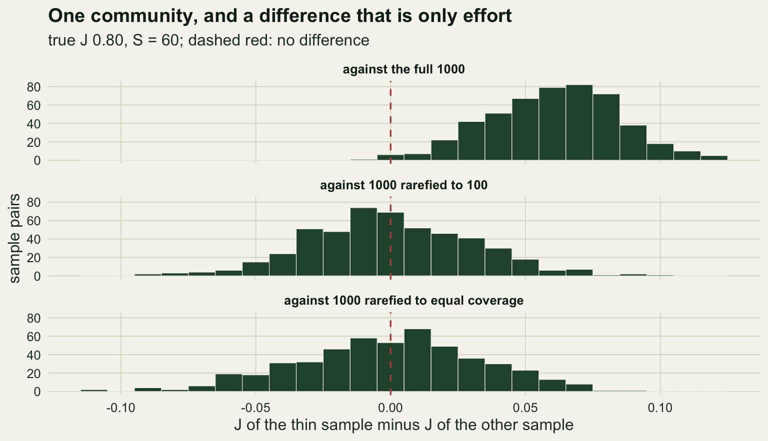
Equal effort does not make richness comparable
Rarefaction works across effort because both samples then lose the same species, in expectation, from the same community. It cannot do that for two communities of different richness: at equal n they lose different shares of their species. The check below is the J version of the beta post’s equal effort section. Two communities have exactly the same true J by construction, one with 40 species and one with 100, sampled at the same n; the denominator is 500 sample pairs per cell, and a difference is declared when the bootstrap interval, built as in the previous section, excludes zero. The coverage arm brings the sample with the higher estimated coverage down to the coverage of the other before the bootstrap.
n_w1 <- 500
set.seed(3731)
w1_tab <- NULL
for (tg in c(0.80, 0.90)) {
  p_40  <- det_sad(40, tune_sd(40, tg))
  p_100 <- det_sad(100, tune_sd(100, tg))
  for (n in c(100, 300)) {
    r_w <- replicate(n_w1, {
      x_a <- rmultinom(1, n, p_40)[, 1]
      x_b <- rmultinom(1, n, p_100)[, 1]
      c_a <- cov_hat(x_a); c_b <- cov_hat(x_b)
      x_ac <- if (c_a > c_b) rarefy_cols(matrix(x_a), m_for_cov(x_a, c_b))[, 1] else x_a
      x_bc <- if (c_b > c_a) rarefy_cols(matrix(x_b), m_for_cov(x_b, c_a))[, 1] else x_b
      j_a <- ev_idx(matrix(x_a))[, "J"];  j_b <- ev_idx(matrix(x_b))[, "J"]
      j_ac <- ev_idx(matrix(x_ac))[, "J"]; j_bc <- ev_idx(matrix(x_bc))[, "J"]
      c(d_n = unname(j_a - j_b), sig_n = excl0(boot_J(x_a) - boot_J(x_b)),
        d_c = unname(j_ac - j_bc), sig_c = excl0(boot_J(x_ac) - boot_J(x_bc)),
        m_a = sum(x_ac), rich_even = unname(j_b > j_a))
    })
    w1_tab <- rbind(w1_tab, data.frame(J_true = tg, n = n, t(rowMeans(r_w))))
  }
}
w1 <- function(tg, n, col) w1_tab[w1_tab$J_true == tg & w1_tab$n == n, col]
w1_max_n <- max(w1_tab$sig_n)
w1_max_c <- max(w1_tab$sig_c)
At equal n the richer community reads as the more even. With both true J at 0.80 and 100 individuals each, J of the 40-species community minus J of the 100-species community averages -0.037, the richer sample has the higher J in 0.896 of pairs, and the interval excludes zero in 0.154. At 300 individuals each the mean difference is -0.030 and the rate rises to 0.296, because the intervals narrow faster than the bias shrinks. At a true J of 0.90 the rates are 0.122 and 0.160. The largest equal-n rate in the four cells, 0.296, is well below the 0.696 of the unequal-effort comparison of one community, which is why size rarefaction is still worth doing: it removes the large problem and leaves a smaller one.
Matching coverage removes most of the smaller one. The mean difference at a true J of 0.80 and 100 individuals falls to -0.004, and the false-difference rate falls to 0.024; the largest coverage-matched rate across the four cells is 0.050. The price is paid in individuals. The 40-species sample, which reaches a given coverage sooner, is cut from 100 individuals to 45.2 on average, and from 300 to 124.9. The beta post found that matching coverage did not rescue its q = 0 turnover between differently structured regions; for J across two richness levels, in this construction, it does most of the job.
That leaves no single standardisation that wins both tests. Size rarefaction ranks two communities of equal richness better; coverage rarefaction is the one that stops a richness difference from posing as an evenness difference. Which of the two situations a survey is in is itself uncertain, because the true richness is not observed.
w1_long <- rbind(
  data.frame(cell = sprintf("true J %.2f, n = %d", w1_tab$J_true, w1_tab$n),
             rate = w1_tab$sig_n, arm = "equal n"),
  data.frame(cell = sprintf("true J %.2f, n = %d", w1_tab$J_true, w1_tab$n),
             rate = w1_tab$sig_c, arm = "equal coverage"))
w1_long$arm  <- factor(w1_long$arm, levels = c("equal n", "equal coverage"))
w1_long$cell <- factor(w1_long$cell, levels = unique(w1_long$cell))
ggplot(w1_long, aes(cell, rate, fill = arm)) +
  geom_col(position = position_dodge(width = 0.75), width = 0.7) +
  geom_hline(yintercept = 0.05, linetype = "dotted", colour = te_body, linewidth = 0.5) +
  geom_hline(yintercept = fd_rate["sig_naive"], linetype = "dashed", colour = te_rust,
             linewidth = 0.6) +
  scale_fill_manual(values = c(te_gold, te_forest), name = NULL) +
  scale_y_continuous(limits = c(0, 0.75)) +
  labs(x = NULL, y = "share of pairs declared different",
       title = "Equal n leaves a richness effect; equal coverage removes most of it",
       subtitle = "dashed red: one community at 100 against 1000, no rarefaction; dotted: 0.05") +
  theme_datasheet() +
  theme(legend.position = "bottom")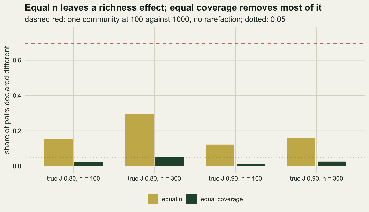
What to report
Do not compare Pielou’s J between samples of different size. If the samples differ in size, rarefy the larger to the size of the smaller before computing J, and average J over many subsamples rather than taking one: in the pond case that moved the share of correct rankings from 0.808 to 0.862, at no cost but computing time. State the n that J was computed at, the way a rarefied richness is stated; rarefied J compares expected J at that n, which for uneven communities compresses a true difference (here the true 0.05 became 0.028 at 100 individuals).
Report the observed richness beside J, and if the two communities differ clearly in observed richness at the common n, report J at equal coverage as well. The two readings answer different worries: equal size protects the ranking of communities that are equally rich, equal coverage protects against a richness difference reading as an evenness difference. If they agree, say so; if they disagree, the evenness difference is not established.
Do not reach for a different evenness index to escape the problem. Heip’s index and Evar were worse than J on unequal samples here, and D2/D1, the index with no richness in it, did worse than H over the log of Chao1, which itself did worse than rarefied J. Heip and Evar both improved once the effort was equalised, and neither improved on rarefied J.
State which way the bias should run for the communities in hand. With 100 individuals against 1000, the thinner sample will look more even below the point where the gap between the two efforts turns: about 0.93 in true J at S = 40, while at S = 100 the gap stayed positive across the whole sweep up to a true J of 0.97, because the bias at 1000 individuals fell further. Above the turning point at S = 40 the reversal is small. A reported evenness difference in the direction the bias predicts deserves the most suspicion.
Honest limits
Every community here is lognormal. A community with a long tail of singletons from a different abundance model, or with a few extreme dominants, would change the size of the bias and could move the turning point; neither case was run. The ranking comparison uses one pair of tuned shapes per contrast, so the rates there carry no between-community variation at all; the random-community grid shows how large that variation is, and it is large.
The samples are multinomial draws of individuals, which is what sampling individuals at random from a well mixed community would give. Real samples are clumped: a kick sample or a trap catch picks up aggregations, and extra-multinomial variation would widen every interval and change the bias in ways this post does not measure. The percentile bootstrap used for the false-difference rates resamples individuals within one sample, and the bootstrap replicates of a thin sample are themselves biased in the direction the post describes, so the interval is not an exact test even after rarefaction; the rarefied rates came out at or below the nominal five per cent in these runs, which is an empirical finding for this setting, not a guarantee.
Coverage matching was done with one construction: the sample with the higher estimated coverage is rarefied to the other’s estimated coverage. That target is itself estimated from a thin sample, and some of the loss of ranking accuracy under coverage matching comes from that noise. Chao and Ricotta’s evenness classes, normalised divergences built from Hill numbers and richness, were not run here, nor any coverage-standardised version of them, and nor was coverage-based extrapolation of the thinner sample.
The richness comparison used 40 against 100 species at two levels of J and two sample sizes. Coverage matching removed most of the effect in those four cells; it does not follow that it removes it for every pair of richness levels or every abundance shape, and the beta post is a reminder that a standardisation built for one quantity can fail for another.
The ranking comparison held richness equal and changed only the shape. Two real communities usually differ in both, so the two failure modes, effort and richness, act together, and their combined effect can add or partly cancel.
References
Heip C 1974 Journal of the Marine Biological Association of the United Kingdom 54(3):555-557 (10.1017/S0025315400022736)
Soetaert K, Heip C 1990 Marine Ecology Progress Series 59:305-307 (10.3354/meps059305)
Smith B, Wilson JB 1996 Oikos 76(1):70-82 (10.2307/3545749)
Chao A, Shen T-J 2003 Environmental and Ecological Statistics 10(4):429-443 (10.1023/A:1026096204727)
Bulinski KV 2007 Palaeogeography, Palaeoclimatology, Palaeoecology 253(3-4):490-508 (10.1016/j.palaeo.2007.06.016)
Chao A, Jost L 2012 Ecology 93(12):2533-2547 (10.1890/11-1952.1)
Chao A, Ricotta C 2019 Ecology 100(12):e02852 (10.1002/ecy.2852)