library(ape)
library(ggplot2)

te_paper  <- "#f5f4ee"
te_ink    <- "#16241d"
te_body   <- "#2c3a31"
te_forest <- "#275139"
te_rust   <- "#b5534e"
te_gold   <- "#c9b458"
te_line   <- "#dad9ca"
te_sage   <- "#93a87f"   # a sixth colour, for the fitted n_eff interval

theme_datasheet <- function() {
  theme_minimal(base_size = 12) +
    theme(plot.background  = element_rect(fill = te_paper, colour = NA),
          panel.background = element_rect(fill = te_paper, colour = NA),
          panel.grid.major = element_line(colour = te_line, linewidth = 0.3),
          panel.grid.minor = element_blank(),
          text             = element_text(colour = te_body),
          plot.title       = element_text(colour = te_ink, face = "bold"),
          plot.subtitle    = element_text(colour = te_body),
          axis.text        = element_text(colour = te_body),
          strip.text       = element_text(colour = te_ink, face = "bold"))
}Phylogeny in a multi-species meta-analysis
R
meta-analysis
phylogenetics
ape
simulation
ecology tutorial
Ignoring the tree shrinks the pooled interval of a multi-species meta-analysis, and the right model still undercovers. Measured in R with ape, plus a t repair.
Forty songbird species, one question: do urban populations lay smaller clutches than rural ones? The synthesis collects a log response ratio of clutch size for each species, urban against rural, from the published studies. In one version of the synthesis every species has been studied in one city pair; in another, every species in three. The pooled mean is the number the abstract will carry, and the confidence interval around it decides whether anyone believes it.
The forty species are not forty independent draws. Two warblers that split from each other a few million years ago share most of their history, including whatever made their clutch size respond to cities in the first place. The standard way to say this in a meta-analysis is a phylogenetic random effect: a species-level effect whose correlation between two species is set by the time they shared on the tree, next to an ordinary species-level effect that carries the part of the response with no phylogenetic pattern. Lajeunesse (2009) set out the phylogenetic version of meta-analysis, and Hadfield and Nakagawa (2010) the model with both species-level terms.
This site has the two halves of that model in separate posts. Dependent effect sizes in meta-analysis handles several effects from one study with a nesting factor, and names the gap in its honest limits: real dependence can come from “a phylogeny, and the last of those needs a correlation matrix rather than a nesting factor”. Phylogenetic generalised least squares shows on a 40-species tree what ignoring the correlation does to a regression slope. The first result below is the same lesson, and it is arithmetic: the interval of a model that treats species as independent can be computed in closed form, and it is too short by a factor this post derives rather than discovers.
The part that is not arithmetic is what happens after the tree is put in. Cinar and colleagues (2022) simulated this family of models and report that, when the phylogenetic relationships are at least moderately strong, only the model with both a phylogenetic and a non-phylogenetic species component gives an approximately unbiased overall mean with confidence intervals close to nominal coverage, while noting that its coverage fell slightly below nominal in most conditions in which all variance components were non-zero. Their trees were random topologies with Grafen branch lengths, and their interval used a t reference on the number of studies minus one. Here the trees are coalescent, the interval is the plain Wald interval most software prints by default, and the measurement is how often it covers the true mean. It falls short. Ancestral state reconstruction in R shows the starting point: the grand mean of a trait evolving on a tree is the estimate at the root, and the root is only ever pinned down loosely. The interval here is short rather than merely wide because the phylogenetic variance that sets its width is itself estimated from one tree, and in a share of fits it is estimated as zero. The last part measures one repair that can be computed from the tree alone, and what it costs.
One tree, forty species, one pooled mean
Each simulated synthesis draws its own tree of forty species from the coalescent with ape::rcoal() and rescales it so that every tip sits at depth one. The Brownian correlation matrix of the tips is then the shared branch length of each pair. Each effect is the true mean, plus a phylogenetic species effect, plus a non-phylogenetic species effect, plus sampling error with a known variance drawn between 0.02 and 0.2, which is the range of a log response ratio from modest studies.
n_sp    <- 40                 # species in the synthesis
mu_true <- 0.3                # true pooled log response ratio
v_lo <- 0.02; v_hi <- 0.2     # range of the known sampling variances
z95  <- qnorm(0.975)
n_rep <- 1000                # syntheses per design, fixed before any run

# three designs, fixed before any coverage was computed
cells <- data.frame(
  label = c("one study per species", "three studies per species",
            "three per species, weak tree"),
  per = c(1, 3, 3),           # effect sizes per species
  s2p = c(0.10, 0.10, 0.03),  # phylogenetic species variance
  s2n = c(0.02, 0.02, 0.10))  # non-phylogenetic species variance

tree_corr <- function(tr) {
  cm <- vcv(tr)
  cm / max(cm)                # Brownian correlation, root-to-tip depth one
}

sim_meta <- function(per, s2p, s2n, tree_fun = rcoal) {
  tr   <- tree_fun(n_sp)
  cmat <- tree_corr(tr)
  sp   <- rep(seq_len(n_sp), each = per)
  v    <- runif(n_sp * per, v_lo, v_hi)
  u    <- drop(crossprod(chol(cmat), rnorm(n_sp))) * sqrt(s2p)
  a    <- rnorm(n_sp, 0, sqrt(s2n))
  list(tr = tr, cmat = cmat, sp = sp, v = v,
       y = mu_true + (u + a)[sp] + rnorm(length(v), 0, sqrt(v)))
}
Two models are fitted to every synthesis, both by restricted maximum likelihood (REML) and both written out in base R. The naive one is the random-effects meta-analysis of Random-effects meta-analysis in R: one between-effect variance, every row independent. The phylogenetic one has the two species-level variances. With no residual variation between studies of the same species beyond sampling error, the precision-weighted mean of each species and its variance carry all the information about the model, so the phylogenetic fit runs on forty species means instead of on every effect; the check below confirms that on a simulated dataset rather than taking it on trust. The variance components are held at or above zero, and a component that wants to be negative stays at exactly zero.
reml_iid <- function(y, v) {
  ll <- function(t2) {
    w <- 1 / (t2 + v); sw <- sum(w); m <- sum(w * y) / sw
    -0.5 * (-sum(log(w)) + log(sw) + sum(w * (y - m)^2))
  }
  o  <- optimize(ll, c(0, max(10 * var(y), 1)), maximum = TRUE, tol = 1e-10)
  t2 <- if (ll(0) >= o$objective) 0 else o$maximum
  w  <- 1 / (t2 + v)
  list(mu = sum(w * y) / sum(w), se = 1 / sqrt(sum(w)), t2 = t2, w = w)
}

# REML log likelihood for V = th[1] * cmat + th[2] * I + diag(d), unknown mean
reml_ll <- function(th, y, d, cmat) {
  vm  <- th[1] * cmat + diag(th[2] + d, length(y))
  ch  <- chol(vm); vi <- chol2inv(ch); vi1 <- rowSums(vi); s <- sum(vi1)
  pm  <- vi - tcrossprod(vi1) / s; py <- drop(pm %*% y)
  list(ll = -0.5 * (2 * sum(log(diag(ch))) + log(s) + sum(y * py)),
       pm = pm, py = py, vi1 = vi1, s = s)
}

# Fisher scoring with the components held at or above zero
reml_phylo <- function(y, d, cmat, th = NULL, tol = 1e-9, maxit = 200) {
  mats <- list(cmat, diag(length(y)))
  if (is.null(th)) th <- rep(max(var(y) - mean(d), 0.01) / 2, 2)
  cur <- reml_ll(th, y, d, cmat)
  for (it in seq_len(maxit)) {
    pmm   <- lapply(mats, function(m) cur$pm %*% m)
    score <- vapply(1:2, function(k) -0.5 * sum(diag(pmm[[k]])) +
                      0.5 * sum(cur$py * (mats[[k]] %*% cur$py)), 0)
    info  <- matrix(0, 2, 2)
    for (k in 1:2) for (l in k:2)
      info[k, l] <- info[l, k] <- 0.5 * sum(pmm[[k]] * t(pmm[[l]]))
    free <- which(th > 0 | score > 0)
    if (!length(free)) break
    step <- rep(0, 2)
    step[free] <- solve(info[free, free, drop = FALSE], score[free])
    h <- 1; ok <- FALSE
    for (j in 1:30) {
      th_new <- pmax(th + h * step, 0); nxt <- reml_ll(th_new, y, d, cmat)
      if (nxt$ll >= cur$ll - 1e-12) { ok <- TRUE; break }
      h <- h / 2
    }
    if (!ok) break
    d_th <- max(abs(th_new - th)); d_ll <- nxt$ll - cur$ll
    th <- th_new; cur <- nxt
    if (d_th < tol || (abs(d_ll) < 1e-12 && d_th < 1e-6)) break
  }
  list(mu = sum(cur$vi1 * y) / cur$s, se = sqrt(1 / cur$s), th = th, ll = cur$ll)
}

species_means <- function(y, v, sp) {
  wt <- as.numeric(rowsum(1 / v, sp))
  list(yb = as.numeric(rowsum(y / v, sp)) / wt, d = 1 / wt)
}
One synthesis with three studies per species shows what the two fits report.
set.seed(45100)
ex <- sim_meta(3, 0.10, 0.02)
ex_naive <- reml_iid(ex$y, ex$v)
ex_sm    <- species_means(ex$y, ex$v, ex$sp)
ex_phylo <- reml_phylo(ex_sm$yb, ex_sm$d, ex$cmat)
ex_ci <- rbind(naive = ex_naive$mu + c(-1, 1) * z95 * ex_naive$se,
               phylo = ex_phylo$mu + c(-1, 1) * z95 * ex_phylo$se)
round(ex_ci, 3)
[,1] [,2]
naive 0.451 0.591
phylo 0.107 0.727The naive fit puts the pooled log response ratio at 0.521 with a standard error of 0.036; its interval runs from 0.451 to 0.591 and excludes zero. The phylogenetic fit on the same 120 effect sizes gives 0.417 with a standard error of 0.158, 4.4 times larger, and an interval from 0.107 to 0.727. The estimated phylogenetic variance is 0.079 and the non-phylogenetic one 0.027, against true values of 0.10 and 0.02.
Before any of that is used, three checks. The tree from rcoal() must be ultrametric so that the rescaled correlation matrix has ones on its diagonal. The species-mean shortcut must give the same REML likelihood surface as the full model on all effects, up to a constant, and the same weighted mean. And the Fisher scoring answer must not be beaten by a general optimiser started elsewhere.
stopifnot(is.ultrametric(ex$tr), isTRUE(all.equal(unname(diag(ex$cmat)), rep(1, n_sp))))

# full model on all effects: V = Z (s2p cmat + s2n I) Z' + diag(v)
zmat <- outer(ex$sp, seq_len(n_sp), "==") * 1
ll_full <- function(th) {
  vm <- zmat %*% (th[1] * ex$cmat + th[2] * diag(n_sp)) %*% t(zmat) + diag(ex$v)
  ch <- chol(vm); vi <- chol2inv(ch); vi1 <- rowSums(vi); s <- sum(vi1)
  r  <- ex$y - sum(vi1 * ex$y) / s
  c(ll = -0.5 * (2 * sum(log(diag(ch))) + log(s) + sum(r * (vi %*% r))),
    mu = sum(vi1 * ex$y) / s)
}
th_a <- c(0.05, 0.01); th_b <- c(0.20, 0.08)
gap_full <- ll_full(th_a)[["ll"]] - ll_full(th_b)[["ll"]]
gap_mean <- reml_ll(th_a, ex_sm$yb, ex_sm$d, ex$cmat)$ll -
            reml_ll(th_b, ex_sm$yb, ex_sm$d, ex$cmat)$ll
mu_gap <- abs(ll_full(ex_phylo$th)[["mu"]] - ex_phylo$mu)
stopifnot(abs(gap_full - gap_mean) < 1e-8, mu_gap < 1e-10)

# a general optimiser from two other starts must not find a higher likelihood
opt_ll <- vapply(list(c(0.01, 0.2), c(0.5, 0.001)), function(s0)
  optim(s0, function(th) -reml_ll(th, ex_sm$yb, ex_sm$d, ex$cmat)$ll,
        method = "L-BFGS-B", lower = c(0, 0))$value, 0)
stopifnot(ex_phylo$ll >= max(-opt_ll) - 1e-6)
All three pass. The likelihood difference between two arbitrary parameter values agrees between the full 120-effect model and the forty species means to within floating-point rounding.
Forty species are worth about three
Under Brownian motion the best estimate of the mean of the tips is the generalised least squares mean, and it is also the estimate at the root. With a unit rate and a tree of depth one its precision is the sum of all entries of the inverse of the tip correlation matrix, sum(solve(cmat)) in R. Call it n_eff: it is the number of independent species that would pin the mean down as well as the whole tree does. Ane (2008) showed that the best linear unbiased estimate of an intercept under Brownian motion on a tree need not become consistent as species are added, and introduced an effective sample size for parameters of that kind. The same precision can be built from the tips down, which shows where it comes from: at each node, every daughter lineage contributes one over its branch length plus the inverse precision below it. The two lineages that meet at the root therefore contribute at most one over their own stem length each, however many species sit above them.
root_precision <- function(tr) {
  tr <- reorder(tr, "postorder"); n <- Ntip(tr)
  bl <- tr$edge.length / max(node.depth.edgelength(tr))
  prec <- c(rep(Inf, n), rep(0, tr$Nnode))
  for (i in seq_len(nrow(tr$edge))) {
    pa <- tr$edge[i, 1]; ch <- tr$edge[i, 2]
    prec[pa] <- prec[pa] + 1 / (bl[i] + 1 / prec[ch])
  }
  stems <- bl[tr$edge[, 1] == n + 1]
  c(prec = prec[n + 1], stem_bound = sum(1 / stems))
}
n_tree <- 1000
set.seed(45105)
neff40 <- t(replicate(n_tree, {
  tr <- rcoal(n_sp); cm <- tree_corr(tr)
  ev <- eigen(cm, symmetric = TRUE, only.values = TRUE)$values
  c(ne = sum(solve(cm)), root_precision(tr), top2 = sum(ev[1:2]) / sum(ev))
}))
prec_gap <- max(abs(neff40[, "ne"] - neff40[, "prec"]))
stopifnot(prec_gap < 1e-8, all(neff40[, "ne"] <= neff40[, "stem_bound"] + 1e-8))
ne_q <- quantile(neff40[, "ne"], c(0.1, 0.5, 0.9))
stem_med <- median(neff40[, "stem_bound"])
below3 <- mean(neff40[, "ne"] < 3)
top2_med <- median(neff40[, "top2"])

sp_grid <- c(10, 20, 40, 80, 160, 320)
n_tree_sweep <- 200
set.seed(45106)
ne_med <- vapply(sp_grid, function(n)
  median(replicate(n_tree_sweep, sum(solve(tree_corr(rcoal(n)))))), 0)
ne_at <- function(n) ne_med[sp_grid == n]
Across 1000 coalescent trees of forty species the matrix formula and the tip-to-root recursion agree to \(4.6 \times 10^{-11}\). The median n_eff is 2.77, with 80 per cent of trees between 2.30 and 3.78. The bound set by the two root stems alone has a median of 3.73, and it holds on every tree. On the grand mean, the median tree of forty species carries the information of fewer than three independent ones, and 64 per cent of the trees carry less than three.
That is a property of the coalescent shape. Its last coalescence is slow, so the two lineages that meet at the root have long stems and every species hangs from one of them. More species hardly change that: the median is 2.60 with ten species, 2.78 with forty and 2.94 with three hundred and twenty.
Ignoring the tree is arithmetic
The naive fit weights each effect by one over its sampling variance plus the estimated between-effect variance, and reports one over the square root of the summed weights as the standard error. Treating those weights as fixed, the true variance of the same weighted mean is the weights times the true covariance matrix of the effects times the weights, divided by the squared sum of the weights. The ratio of the true to the reported standard error follows, and so does the coverage a z interval can reach: twice the normal probability below 1.96 divided by that ratio, minus one. Nothing about it needs simulation. The simulation below computes it for every synthesis and sets it beside the coverage actually observed.
The main run fits both models to 1000 syntheses in each of three designs: one study per species; three studies per species with the same variances; and three studies per species with a weak phylogenetic component, where the non-phylogenetic species variance is the larger one. Each synthesis also gets the generalised least squares interval computed with the true covariance matrix, an oracle that checks the code rather than offering a method.
one_rep <- function(per, s2p, s2n, n_boot = 0, tree_fun = rcoal) {
  dd <- sim_meta(per, s2p, s2n, tree_fun); cmat <- dd$cmat; eye <- diag(n_sp)
  nv <- reml_iid(dd$y, dd$v)
  zw <- as.numeric(rowsum(nv$w, dd$sp))
  true_var <- drop(crossprod(zw, (s2p * cmat + s2n * eye) %*% zw)) + sum(nv$w^2 * dd$v)
  ratio <- sqrt(true_var) / sum(nv$w) / nv$se
  sm <- species_means(dd$y, dd$v, dd$sp)
  f  <- reml_phylo(sm$yb, sm$d, cmat)
  vt_inv <- solve(s2p * cmat + s2n * eye + diag(sm$d))
  s_or <- sum(vt_inv); mu_or <- sum(vt_inv %*% sm$yb) / s_or
  ne_tree <- sum(solve(cmat))
  v_fit <- f$th[1] * cmat + f$th[2] * eye + diag(sm$d)
  ne_fit <- sum(solve(cov2cor(v_fit)))
  q_tree <- qt(0.975, max(ne_tree - 1, 1)); q_fit <- qt(0.975, max(ne_fit - 1, 1))
  out <- c(naive = abs(nv$mu - mu_true) < z95 * nv$se, naive_w = 2 * z95 * nv$se,
    ratio = ratio, naive_pred = 2 * pnorm(z95 / ratio) - 1,
    wald = abs(f$mu - mu_true) < z95 * f$se, wald_w = 2 * z95 * f$se,
    fit_t = abs(f$mu - mu_true) < q_fit * f$se, fit_t_w = 2 * q_fit * f$se,
    tree_t = abs(f$mu - mu_true) < q_tree * f$se, tree_t_w = 2 * q_tree * f$se,
    oracle = abs(mu_or - mu_true) < z95 / sqrt(s_or), oracle_w = 2 * z95 / sqrt(s_or),
    ne_tree = ne_tree, ne_fit = ne_fit, s2p_hat = f$th[1],
    at_zero = f$th[1] < 1e-6, err = f$mu - mu_true, boot_t = NA, boot_t_w = NA)
  if (n_boot > 0) {           # parametric bootstrap-t from the fitted model
    lo_tri <- t(chol(v_fit))
    ystar <- f$mu + lo_tri %*% matrix(rnorm(n_sp * n_boot), n_sp, n_boot)
    tstar <- apply(ystar, 2, function(ys) {
      g <- reml_phylo(ys, sm$d, cmat, th = pmax(f$th, 1e-4)); (g$mu - f$mu) / g$se })
    tq <- sort(tstar); k <- round(0.025 * (n_boot + 1))
    lo <- f$mu - tq[n_boot + 1 - k] * f$se; hi <- f$mu - tq[k] * f$se
    out[c("boot_t", "boot_t_w")] <- c(lo < mu_true & hi > mu_true, hi - lo)
  }
  out
}
cell_seeds <- c(45101, 45102, 45103)
runs <- lapply(seq_len(nrow(cells)), function(j) {
  set.seed(cell_seeds[j])
  t(replicate(n_rep, one_rep(cells$per[j], cells$s2p[j], cells$s2n[j])))
})
cov_of <- function(j, m) mean(runs[[j]][, m])
wid_of <- function(j, m) median(runs[[j]][, paste0(m, "_w")])
mcse_of <- function(p, n = n_rep) sqrt(p * (1 - p) / n)
ratio_med  <- vapply(1:3, function(j) median(runs[[j]][, "ratio"]), 0)
naive_pred <- vapply(1:3, function(j) mean(runs[[j]][, "naive_pred"]), 0)
naive_obs  <- vapply(1:3, function(j) cov_of(j, "naive"), 0)
pred_gap   <- max(abs(naive_pred - naive_obs) / mcse_of(naive_obs))
Ignoring the tree, the reported standard error is too small by a median factor of 3.56 with one study per species, 6.06 with three and 3.15 with three studies and a weak phylogenetic component. The interval is a third to a sixth of the width it should be. The closed form predicts coverage of 0.427, 0.263 and 0.469; the simulation observes 0.406, 0.260 and 0.473, and the largest gap is 1.4 Monte Carlo standard errors. The naive failure is the formula, and the PGLS post already made the same point for a slope.
The second design is the one that bites in practice. Tripling the studies per species triples the rows and the naive weights, so the naive interval shrinks from a median width of 0.243 to 0.140, while nothing has been learned about the phylogenetic part of the mean. Its coverage drops with it.
The right model still falls short
The phylogenetic model has the right covariance structure and estimates the mean without bias: across the first design the mean error of the pooled estimate is -0.0034, against a standard deviation of 0.201. Its Wald interval, the one printed by default, is another matter.
wald_cov <- vapply(1:3, function(j) cov_of(j, "wald"), 0)
at0   <- vapply(1:3, function(j) mean(runs[[j]][, "at_zero"]), 0)
split_cov <- t(vapply(1:3, function(j) {
  b <- runs[[j]][, "at_zero"] == 1
  c(boundary = mean(runs[[j]][b, "wald"]), interior = mean(runs[[j]][!b, "wald"]),
    n_b = sum(b))
}, numeric(3)))
miss_share <- (at0 * (1 - split_cov[, "boundary"])) / (1 - wald_cov)
stopifnot(all(split_cov[, "n_b"] >= 30))
With one study per species the Wald interval covers the true mean in 0.804 of syntheses; with three it covers 0.833, and with the weak tree 0.833, each with a Monte Carlo standard error of at most 0.013. That is far better than ignoring the tree and still well short of 0.95.
The mechanism is the estimate of the phylogenetic variance. It is estimated from one tree, and most of the phylogenetic variation among the tips runs along a few deep splits: across the thousand trees above, the two largest eigenvalues of the tip correlation matrix hold a median of 76 per cent of its trace. The data offer only a few independent looks at that variance, and in 13.4 per cent of the first design’s fits it lands exactly on zero (5.8 and 32.4 per cent in the other two). A fit with no phylogenetic variance treats the species as independent up to their non-phylogenetic term, and its interval inherits the naive problem. Those fits cover the true mean only 0.328, 0.172 and 0.651 of the time, and in the first design they supply 46 per cent of all the misses. The interior fits cover 0.878, 0.874 and 0.920: better, and still short, in part because a z interval ignores the uncertainty in the variance components it was built from. The same boundary appears for a single between-site variance in Prediction intervals for a new site in meta-analysis, where an estimate of exactly zero collapses the interval.
split_d <- data.frame(
  design = factor(rep(c("one per\nspecies", "three per\nspecies", "weak\ntree"), 2),
                  levels = c("one per\nspecies", "three per\nspecies", "weak\ntree")),
  state = factor(rep(c("estimate on zero", "positive estimate"), each = 3),
                 levels = c("estimate on zero", "positive estimate")),
  cover = c(split_cov[, "boundary"], split_cov[, "interior"]))
ggplot(split_d, aes(design, cover, fill = state)) +
  geom_col(position = position_dodge(width = 0.75), width = 0.65) +
  geom_hline(yintercept = 0.95, colour = te_body, linetype = "dashed", linewidth = 0.5) +
  scale_fill_manual(values = c(te_rust, te_forest), name = NULL) +
  scale_y_continuous(limits = c(0, 1)) +
  labs(x = NULL, y = "Wald coverage", title = "Zero fits drag it down",
       subtitle = "dashed line: nominal 0.95") +
  theme_datasheet() + theme(legend.position = "bottom")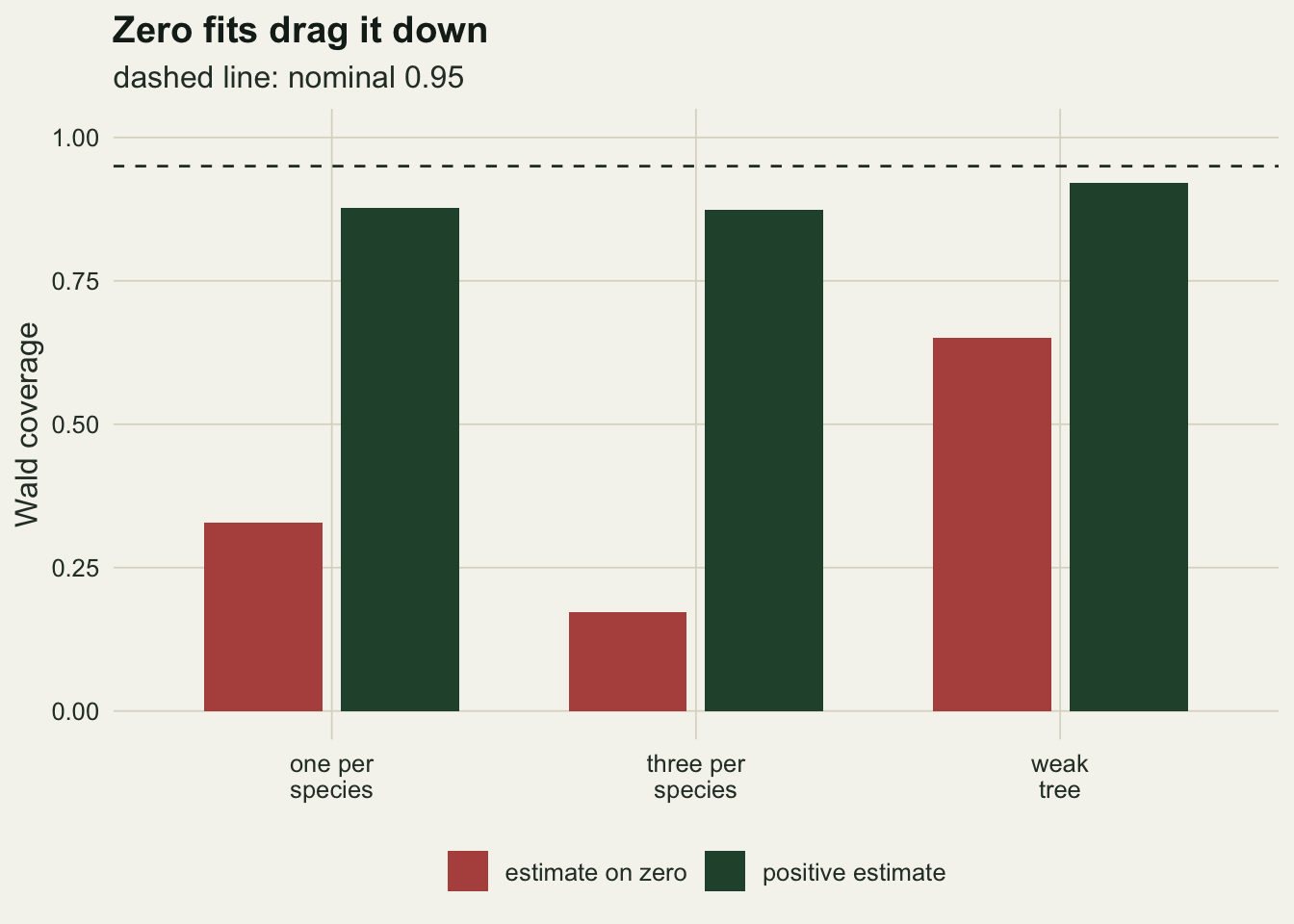
Counting the tree’s degrees of freedom
The count of lineages does not give the degrees of freedom of an exact interval. If the variance were purely phylogenetic, with a known correlation matrix and only the Brownian rate unknown, generalised least squares would turn the tree into forty independent pieces, and the exact interval would be a t on n - 1 = 39 degrees of freedom. A quick check on trees like the ones above:
n_bm <- 2000
set.seed(45107)
bm_cov <- rowMeans(replicate(n_bm, {
  cmat <- tree_corr(rcoal(n_sp)); ci <- solve(cmat); s <- sum(ci)
  y  <- mu_true + drop(crossprod(chol(cmat), rnorm(n_sp))) * sqrt(0.10)
  m  <- sum(ci %*% y) / s; r <- y - m
  se <- sqrt(drop(r %*% ci %*% r) / (n_sp - 1) / s)
  c(t39 = abs(m - mu_true) < qt(0.975, n_sp - 1) * se,
    z   = abs(m - mu_true) < z95 * se,
    t_ne = abs(m - mu_true) < qt(0.975, max(s - 1, 1)) * se)
}))
Over 2000 trees the t on 39 degrees of freedom covers 0.948, the z interval 0.940, and a t on n_eff - 1 degrees of freedom 1.000. In this case, which has an exact answer, the t on 39 degrees of freedom is the right interval and the count of lineages is far too cautious. The trouble in this post comes from the two variance components estimated alongside the mean, not from the tree alone.
The repair tried here borrows a looser idea: the grand mean rests on about n_eff independent lineages, so its interval gets no more degrees of freedom than that. Keep the phylogenetic fit and its standard error, and replace 1.96 by the 97.5th percentile of a t on n_eff - 1 degrees of freedom, with n_eff computed from the tree alone. It is a heuristic, not a derivation, and it was fixed before the coverage runs, together with one alternative: the same t with n_eff computed from the correlation matrix of the fitted covariance, which adds in the independent information carried by the non-phylogenetic and sampling variance.
tree_cov <- vapply(1:3, function(j) cov_of(j, "tree_t"), 0)
fit_cov  <- vapply(1:3, function(j) cov_of(j, "fit_t"), 0)
w_tab <- sapply(c("naive", "wald", "fit_t", "tree_t", "oracle"),
                function(m) vapply(1:3, function(j) wid_of(j, m), 0))
ne_fit_med <- vapply(1:3, function(j) median(runs[[j]][, "ne_fit"]), 0)
b1 <- runs[[1]][, "at_zero"] == 1
ne_fit_split <- c(boundary = median(runs[[1]][b1, "ne_fit"]), interior = median(runs[[1]][!b1, "ne_fit"]))
q_med <- qt(0.975, median(runs[[1]][, "ne_tree"]) - 1)
tree_split <- t(vapply(1:3, function(j) {
  b <- runs[[j]][, "at_zero"] == 1
  c(boundary = mean(runs[[j]][b, "tree_t"]), interior = mean(runs[[j]][!b, "tree_t"]))
}, numeric(2)))
With n_eff from the tree the interval covers 0.975 with one study per species and 0.970 with three. The price is width. At the median tree the multiplier is 5.03 instead of 1.96, and the median interval in the first design is 1.62 wide, against 0.68 for the Wald interval and 0.80 for the oracle that knows the true covariance: 2.0 times the oracle width. Where the phylogenetic share is small the repair over-covers, at 0.990, because the tree then understates how much independent information the species carry. This is a conservative interval on average, not a calibrated one. The average hides the same split as the Wald interval. Where the phylogenetic variance was estimated as zero, the repair covers 0.866, 0.655 and 0.972 in the three designs; where it was positive, 0.992, 0.989 and 0.999. It over-covers the interior fits, and that makes up for the boundary fits on average. A zero estimate still leaves the repaired interval short in the first two designs.
The pre-specified alternative fails. Counting n_eff from the fitted covariance gives a median of 7.3 effective species in the first design and coverage of 0.830, 0.882 and 0.846. It fails for the same reason the Wald interval does: when the fitted phylogenetic variance is zero, the fitted covariance has no tree in it, and the count comes out large exactly when it should be small: in the first design its median is 40.0 in the fits on zero and 6.5 in the others.
meth_col <- c(te_rust, te_gold, te_sage, te_forest, te_ink)
meth_lab <- c(naive = "ignore the tree", wald = "phylogenetic, Wald",
              fit_t = "t, fitted n_eff", tree_t = "t, tree n_eff",
              oracle = "oracle, true V")
cov_d <- do.call(rbind, lapply(1:3, function(j) data.frame(
  design = cells$label[j], method = names(meth_lab),
  cover = vapply(names(meth_lab), function(m) cov_of(j, m), 0))))
cov_d$design <- factor(cov_d$design, levels = cells$label)
cov_d$method <- factor(meth_lab[cov_d$method], levels = rev(meth_lab))
cov_d$se <- mcse_of(cov_d$cover)
p_cov <- ggplot(cov_d, aes(cover, method, colour = method)) +
  geom_vline(xintercept = 0.95, colour = te_body, linetype = "dashed", linewidth = 0.5) +
  geom_errorbar(aes(xmin = cover - 2 * se, xmax = cover + 2 * se),
                orientation = "y", width = 0.3, linewidth = 0.5) +
  geom_point(size = 2.6) +
  facet_wrap(~ design, ncol = 3) +
  scale_colour_manual(values = rev(meth_col),
                      guide = "none") +
  scale_x_continuous(limits = c(0.2, 1), breaks = c(0.25, 0.5, 0.75, 0.95)) +
  labs(x = "coverage of the true pooled mean", y = NULL,
       title = "Of the usable intervals, only the tree-count t reaches 0.95",
       subtitle = "dashed line: nominal 0.95") +
  theme_datasheet() + theme(panel.spacing = unit(1.6, "lines"))
p_cov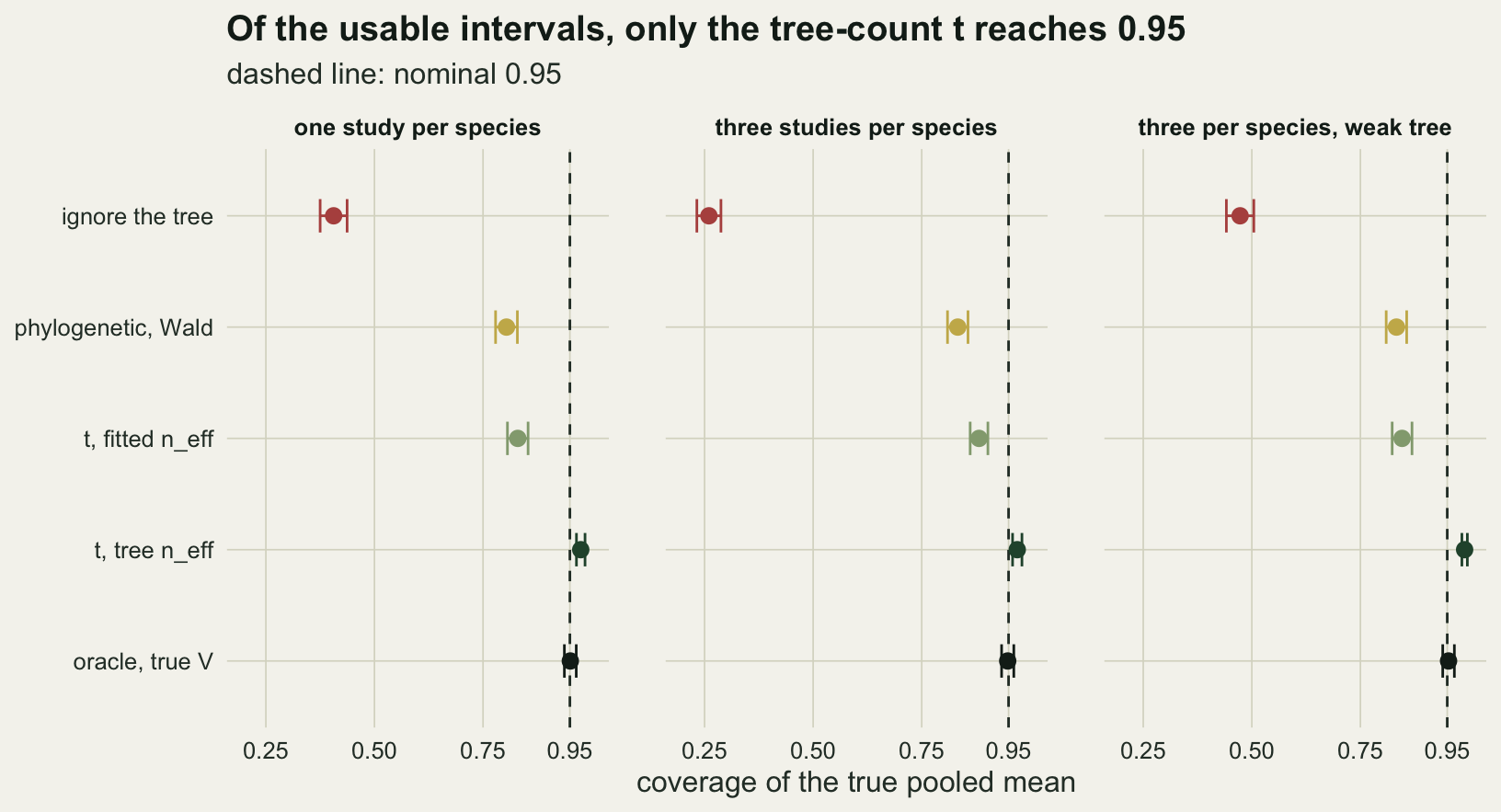
A parametric bootstrap is the other obvious repair: simulate new syntheses from the fitted model on the same tree, refit each, and use the spread of the studentised estimates. It is much slower, so it is run on the first design only.
n_boot_rep <- 200; n_boot <- 199   # fixed before the run
set.seed(45104)
bt <- t(replicate(n_boot_rep, one_rep(1, 0.10, 0.02, n_boot = n_boot)))
bt_zero <- bt[, "at_zero"] == 1
bt_cov <- c(all = mean(bt[, "boot_t"]), boundary = mean(bt[bt_zero, "boot_t"]),
            interior = mean(bt[!bt_zero, "boot_t"]), wald = mean(bt[, "wald"]))
bt_w <- median(bt[, "boot_t_w"])
stopifnot(sum(bt_zero) >= 10)
Over 200 syntheses with 199 bootstrap refits each, the bootstrap-t interval covers 0.900, with a Monte Carlo standard error of 0.021; the Wald interval on the same syntheses covers 0.835. Split by the fit, the bootstrap covers 0.954 where the phylogenetic variance was positive and 0.538 in the 26 syntheses where it was zero. The second number is the limit of any bootstrap from the fitted model: a fitted world with no phylogenetic variance cannot simulate the variance it is missing. Its median width is 1.36, not far below the tree-count t at 1.62, and it costs 199 refits per synthesis.
The trees so far are all coalescent. The same first design on two other shapes, random topologies with Grafen branch lengths and pure-birth (Yule) trees, shows how much of the result belongs to the tree shape.
shape_fun <- list(Grafen = function(n) compute.brlen(rtree(n)),
                  Yule   = function(n) rphylo(n, 1, 0))
stopifnot(all(vapply(shape_fun, function(f) is.ultrametric(f(n_sp)), TRUE)))
n_shape <- 1000
shape_tab <- sapply(seq_along(shape_fun), function(k) {
  set.seed(45107 + k)
  r <- t(replicate(n_shape, one_rep(1, 0.10, 0.02, tree_fun = shape_fun[[k]])))
  b <- r[, "at_zero"] == 1
  c(ne = median(r[, "ne_tree"]), at0 = mean(b), wald = mean(r[, "wald"]),
    tree_t = mean(r[, "tree_t"]), tree_b = mean(r[b, "tree_t"]),
    tree_i = mean(r[!b, "tree_t"]), oracle = mean(r[, "oracle"]),
    ratio = median(r[, "tree_t_w"] / r[, "oracle_w"]))
})
colnames(shape_tab) <- names(shape_fun)
round(shape_tab, 3)
Grafen Yule
ne 3.246 4.932
at0 0.081 0.087
wald 0.858 0.884
tree_t 0.963 0.954
tree_b 0.802 0.724
tree_i 0.977 0.976
oracle 0.946 0.955
ratio 1.681 1.339The median n_eff is 3.25 on the Grafen trees and 4.93 on the Yule trees, against 2.77 on the coalescent. The Wald interval covers 0.858 and 0.884, the tree-count t 0.963 and 0.954, and the oracle 0.946 and 0.955, each with a Monte Carlo standard error of at most 0.011. On the Yule trees the repair sits at nominal on average rather than above it. The median ratio of its width to the oracle’s is 1.68 and 1.34, against 2.07 on the coalescent trees. The split by the fit holds on both shapes: where the phylogenetic variance was estimated as zero (8.1 and 8.7 per cent of fits) the repair covers 0.802 and 0.724, and elsewhere 0.977 and 0.976.
Three studies per species do not narrow it
The width of the correct interval is set by the tree, not by the number of rows.
From one study per species to three, the median Wald width goes from 0.679 to 0.697, the oracle width from 0.799 to 0.776, and the naive width from 0.243 to 0.140. The two t intervals widen instead: the tree-count t from 1.617 to 1.696 and the t on the fitted count from 0.838 to 1.066. Extra studies of the same species sharpen each species mean, but the uncertainty that dominates the grand mean sits in the phylogenetic variance, which the extra rows do not touch. With the weak tree the Wald interval is 0.383 wide, and the tree-count t 0.959, 2.0 times the oracle.
What to report
Report the tree and how its branch lengths were made, because the correlation matrix is part of the model. Report both species-level variances, and say plainly when the phylogenetic one was estimated as zero: that is the state in which both the default and the repaired interval are least trustworthy, not a sign that phylogeny does not matter.
Report n_eff next to the number of species. It takes one line, sum(solve(cmat)) on the correlation matrix of an ultrametric tree rescaled to depth one, and a reader who sees forty species and an effective count near three knows at once how much the grand mean can say.
If the pooled mean is the headline, give the interval with a t reference on n_eff - 1 degrees of freedom alongside the default. Call it conservative on average for coalescent-like trees, not in general: on the Yule trees above it was at nominal, and in fits with a zero phylogenetic variance it fell short in both designs with a strong phylogenetic component and on every tree shape tried. In metafor (Viechtbauer 2010) the same model and the repair look like this; the chunk is not run on this page, and was checked while writing it against metafor 4.4.0, where dfs also accepts a number.
library(metafor)
cmat <- vcv(tree); cmat <- cmat / max(cmat)   # rows and columns named by species
ne   <- sum(solve(cmat))
fit <- rma.mv(yi, vi, random = list(~ 1 | phylo, ~ 1 | species),
              R = list(phylo = cmat), data = dat, test = "t", dfs = ne - 1)
With test = "t" alone, rma.mv() uses the number of effect sizes minus the number of fixed coefficients as its degrees of freedom, and with dfs = "contain" it uses a count at the species level; neither knows about the tree, and both are far above n_eff here.
In these runs, extra studies of already sampled species did not narrow the correct interval. Extra species raise n_eff only slowly, and the root-stem bound says where the gain can come from: lineages that join the tree near the root.
Honest limits
The main runs use coalescent trees rescaled to depth one. The coalescent has long root stems, which is why n_eff is so small. The Grafen and Yule runs give larger counts, and on the Yule trees an average coverage for the repair at nominal rather than above it, but they cover only the first design, with a thousand syntheses each; the other designs on those shapes, and other shapes altogether, were not measured. Real trees are also estimated, and error in the branch lengths near the root moves n_eff directly.
The t repair is not calibrated. On coalescent trees it covers above nominal on average in all three designs, most where the non-phylogenetic variance dominates, and its interval is about twice the oracle width; on Yule trees it sits at nominal. In the fits where the phylogenetic variance was estimated as zero it covers below nominal in the first two designs and on every tree shape tried; only in the weak-tree design did those fits reach nominal. A better interval probably needs a likelihood that treats the variance components as uncertain, a profile or Bayesian interval, and none was measured here.
The model has no study level: each species’ studies differ only by sampling error. With residual variation between studies of the same species, the species-mean shortcut used for speed no longer holds and a fourth variance component enters; the direction of the boundary problem should be the same, but its size was not measured. There is also a single overall mean and no moderator, and the sampling variances are treated as known.
The Monte Carlo standard error is at most 1.6 percentage points for the main runs and 3.5 for the bootstrap, which ran on one design with 200 syntheses. The boundary and interior splits rest on fewer fits than that, and their numbers are correspondingly rougher.
References
Lajeunesse MJ 2009 The American Naturalist 174(3):369-381 (10.1086/603628)
Hadfield JD, Nakagawa S 2010 Journal of Evolutionary Biology 23(3):494-508 (10.1111/j.1420-9101.2009.01915.x)
Cinar O, Nakagawa S, Viechtbauer W 2022 Methods in Ecology and Evolution 13(2):383-395 (10.1111/2041-210X.13760)
Ane C 2008 The Annals of Applied Statistics 2(3):1078-1102 (10.1214/08-AOAS173)
Viechtbauer W 2010 Journal of Statistical Software 36(3):1-48 (10.18637/jss.v036.i03)