library(ggplot2)
library(patchwork)

te_paper  <- "#f5f4ee"
te_ink    <- "#16241d"
te_body   <- "#2c3a31"
te_forest <- "#275139"
te_rust   <- "#b5534e"
te_gold   <- "#c9b458"
te_line   <- "#dad9ca"

theme_datasheet <- function() {
  theme_minimal(base_size = 12) +
    theme(plot.background  = element_rect(fill = te_paper, colour = NA),
          panel.background = element_rect(fill = te_paper, colour = NA),
          panel.grid.major = element_line(colour = te_line, linewidth = 0.3),
          panel.grid.minor = element_blank(),
          text             = element_text(colour = te_body),
          plot.title       = element_text(colour = te_ink, face = "bold"),
          plot.subtitle    = element_text(colour = te_body),
          axis.text        = element_text(colour = te_body))
}Prediction intervals for a new site in meta-analysis
R
meta-analysis
heterogeneity
simulation
ecology tutorial
A random-effects prediction interval is meant to cover the effect at a new site 95 per cent of the time. Measured in R across study counts, tau and estimators.
A grassland manager is deciding whether to fence livestock out of a set of degraded meadows. A published synthesis has pooled twenty exclosure experiments and reports a standardised mean difference in plant species richness, with a confidence interval for the mean that sits well clear of zero. The manager’s question is not about the mean of twenty past sites. It is whether fencing will raise richness at her site, which is not one of the twenty. The interval that is meant to answer that question is the prediction interval: the pooled mean plus and minus a multiple of the square root of the between-site variance plus the squared standard error of the mean.
This site has two posts that meet this interval. Heterogeneity in meta-analysis computes it for one simulated set of eighteen studies, calls its width the honest statement of how much a new study might differ, and moves on. Random-effects meta-analysis in R runs a coverage check, but the target there is the mean effect, not the effect at a fresh site. Neither asks whether the prediction interval covers a new site’s true effect as often as it claims. That is what this post measures, at the numbers of studies ecological syntheses have, with the between-site spread varied from barely there to large.
The answer is not new. Partlett and Riley 2017 simulated exactly this coverage after REML estimation. They found prediction intervals valid only when between-study heterogeneity was large or study sizes similar, and found that when heterogeneity was small and study sizes varied, neither adding studies nor changing the degrees of freedom improved coverage consistently. The interval with a t distribution on k minus two degrees of freedom, the version used here, was proposed by Higgins, Thompson and Spiegelhalter 2009, and IntHout and colleagues 2016 made the case for reporting it. What follows is a demonstration of their result in base R, on a Hedges g scale with the small, unequal sample sizes of field experiments, followed by the parts a reader of a synthesis needs next: why the interval misses, whether a different estimator of the between-site variance or a bootstrap repairs it, what more studies do, and what changes when the thing to be predicted is an observed replicate at a new site rather than its true effect. The post on reference sites and tolerance bounds asks a related question about one set of sites, where the guarantee a bound gives belongs to the reference set it was built from; the same distinction between average and per-synthesis coverage turns up below.
A synthesis and the interval it reports
Each simulated study is a two-arm experiment with between 8 and 40 plots per arm. Its true effect is drawn from a normal distribution with mean 0.3 and standard deviation tau, the between-site spread, and its Hedges g and the usual large-sample variance are computed from the arms. The pooled mean and tau-squared use the DerSimonian and Laird 1986 moment estimator, written out in base R.
mu_true  <- 0.3                      # mean true effect, Hedges g
n_lo     <- 8; n_hi <- 40            # plots per arm, drawn uniformly
k_grid   <- c(5, 10, 20, 40, 80)     # studies in a synthesis
tau_grid <- c(0.05, 0.15, 0.3, 0.5)  # between-site standard deviation
n_rep    <- 2000                     # syntheses per cell, fixed before any run

# draw the sufficient statistics of two normal arms: the mean difference is
# normal and the pooled variance is an independent scaled chi-squared variate
draw_g <- function(theta, n_arm) {
  mdiff <- rnorm(length(theta), theta, sqrt(2 / n_arm))
  s2    <- rchisq(length(theta), 2 * n_arm - 2) / (2 * n_arm - 2)
  (1 - 3 / (8 * n_arm - 9)) * mdiff / sqrt(s2)
}

sim_syntheses <- function(n_syn, k, tau, generator = "arms") {
  n_arm <- matrix(sample(n_lo:n_hi, n_syn * k, replace = TRUE), n_syn, k)
  theta <- rnorm(n_syn * k, mu_true, tau)
  if (generator == "normal") {
    v <- 2 / n_arm + mu_true^2 / (4 * n_arm)     # normal effects, variance known
    g <- matrix(rnorm(n_syn * k, theta, sqrt(v)), n_syn, k)
  } else {
    g <- matrix(draw_g(theta, n_arm), n_syn, k)
    v <- if (generator == "arms") 2 / n_arm + g^2 / (4 * n_arm)   # as a synthesis computes it
         else 2 / n_arm + mu_true^2 / (4 * n_arm)                 # "arms_mu": true mean plugged in
  }
  list(g = g, v = v)
}

q_gen <- function(g, v, tau2) {
  w <- 1 / (v + tau2)
  m <- rowSums(w * g) / rowSums(w)
  rowSums(w * (g - m)^2)
}
tau2_dl <- function(g, v) {
  w <- 1 / v
  pmax(0, (q_gen(g, v, 0) - (ncol(g) - 1)) / (rowSums(w) - rowSums(w^2) / rowSums(w)))
}
pool <- function(g, v, tau2) {
  w <- 1 / (v + tau2)
  list(m = rowSums(w * g) / rowSums(w), se = sqrt(1 / rowSums(w)))
}
# exact share of new sites whose true effect falls inside [lo, hi]
cond_cover <- function(lo, hi, tau) pnorm((hi - mu_true) / tau) - pnorm((lo - mu_true) / tau)
Every function works on a matrix with one synthesis per row, so a whole cell of the simulation is a handful of matrix operations. Drawing the mean difference and the pooled variance instead of every plot is exact for normal arms.
set.seed(2026)
k_ex <- 20; tau_ex <- 0.15
ex <- sim_syntheses(1, k_ex, tau_ex)
ex_tau2 <- tau2_dl(ex$g, ex$v)
ex_fit  <- pool(ex$g, ex$v, ex_tau2)
ex_ci   <- ex_fit$m + c(-1, 1) * qnorm(0.975) * ex_fit$se
ex_pi   <- ex_fit$m + c(-1, 1) * qt(0.975, k_ex - 2) * sqrt(ex_tau2 + ex_fit$se^2)
ex_cov  <- cond_cover(ex_pi[1], ex_pi[2], tau_ex)
ex_need <- 2 * qnorm(0.975) * tau_ex
One synthesis of 20 studies with a true tau of 0.15: the pooled mean is 0.265, tau-squared is estimated at 0.0000 (the truncated estimate) against a true 0.0225, the confidence interval for the mean runs from 0.139 to 0.392 and the prediction interval from 0.130 to 0.401. Because the simulation knows the distribution of true site effects, the share of all possible new sites that this particular interval covers can be computed exactly rather than sampled: it is 0.621. An interval that knew the truth would need a width of 0.588 to cover 95 per cent of sites; this one is 0.271 wide.
Coverage across the syntheses ecologists have
The same exact calculation, averaged over 2000 syntheses per cell, is the coverage of the procedure. It equals the rate at which the interval would contain one freshly drawn site per synthesis, with a smaller Monte Carlo error, and that equality is checked in the chunk. Six intervals are scored on the same syntheses; this section uses the DerSimonian-Laird interval with a normal multiplier, the same with t on k minus two degrees of freedom, and the confidence interval for the mean read as if it were a forecast for a site. The other three enter in the section on estimators.
# generalised Q equal to a target: Paule-Mandel (target k - 1) and the
# Q-profile upper bound for tau-squared (target the lower 2.5 per cent point)
tau2_qsolve <- function(g, v, target, upper = 10, n_iter = 60) {
  lo_b <- rep(0, nrow(g)); hi_b <- rep(upper, nrow(g))
  for (i in seq_len(n_iter)) {
    mid <- (lo_b + hi_b) / 2
    above <- q_gen(g, v, mid) > target
    lo_b[above] <- mid[above]; hi_b[!above] <- mid[!above]
  }
  ifelse(q_gen(g, v, 0) <= target, 0, (lo_b + hi_b) / 2)
}
# REML by its fixed-point equation, truncated at zero
tau2_reml <- function(g, v, n_iter = 300) {
  tau2 <- tau2_dl(g, v)
  for (i in seq_len(n_iter)) {
    w <- 1 / (v + tau2); m <- rowSums(w * g) / rowSums(w)
    tau2 <- pmax(0, rowSums(w^2 * ((g - m)^2 - v)) / rowSums(w^2) + 1 / rowSums(w))
  }
  tau2
}
The Paule-Mandel solver bisects on the generalised Q, and REML is found by its fixed-point equation; both return a whole column of estimates at once.
score_cell <- function(k, tau) {
  s <- sim_syntheses(n_rep, k, tau); g <- s$g; v <- s$v
  t_dl <- tau2_dl(g, v); t_pm <- tau2_qsolve(g, v, k - 1)
  t_reml <- tau2_reml(g, v); t_up <- tau2_qsolve(g, v, qchisq(0.025, k - 1))
  f_dl <- pool(g, v, t_dl); f_pm <- pool(g, v, t_pm)
  f_reml <- pool(g, v, t_reml); f_up <- pool(g, v, t_up)
  crit_t <- qt(0.975, k - 2); crit_z <- qnorm(0.975)
  half <- cbind(dl_z   = crit_z * sqrt(t_dl + f_dl$se^2),
                dl_t   = crit_t * sqrt(t_dl + f_dl$se^2),
                pm_t   = crit_t * sqrt(t_pm + f_pm$se^2),
                reml_t = crit_t * sqrt(t_reml + f_reml$se^2),
                qp_t   = crit_t * sqrt(t_up + f_up$se^2),
                ci_z   = crit_z * f_dl$se)
  centre <- cbind(f_dl$m, f_dl$m, f_pm$m, f_reml$m, f_up$m, f_dl$m)
  cc <- cond_cover(centre - half, centre + half, tau)
  site <- rnorm(n_rep, mu_true, tau)
  list(tab = data.frame(k = k, tau = tau, interval = colnames(half),
                        coverage = colMeans(cc), mcse = apply(cc, 2, sd) / sqrt(n_rep),
                        one_site = colMeans(abs(site - centre) <= half),
                        width = colMeans(2 * half), below90 = colMeans(cc < 0.90),
                        zero = mean(t_dl == 0), zero_reml = mean(t_reml == 0),
                        cc_zero = mean(cc[t_dl == 0, "dl_t"])),
       cc_dl_t = cc[, "dl_t"], zero_dl = t_dl == 0)
}
set.seed(4410)
cells <- expand.grid(k = k_grid, tau = tau_grid)
runs  <- lapply(seq_len(nrow(cells)), function(j) score_cell(cells$k[j], cells$tau[j]))
grid_tab <- do.call(rbind, lapply(runs, `[[`, "tab"))
rownames(grid_tab) <- NULL
cv <- function(k, tau, iv = "dl_t", col = "coverage")
  grid_tab[grid_tab$k == k & grid_tab$tau == tau & grid_tab$interval == iv, col]
site_gap  <- max(abs(grid_tab$one_site - grid_tab$coverage) /
                 sqrt(grid_tab$coverage * (1 - grid_tab$coverage) / n_rep + 1e-12))
mcse_max  <- max(grid_tab$mcse[grid_tab$interval == "dl_t"])
dlt <- grid_tab[grid_tab$interval == "dl_t", ]
dlt_min <- min(dlt$coverage); dlt_min_k <- dlt$k[which.min(dlt$coverage)]
dlt_min_tau <- dlt$tau[which.min(dlt$coverage)]
ci_k40 <- range(grid_tab$coverage[grid_tab$interval == "ci_z" & grid_tab$k == 40])
At tau 0.05, a between-site spread that is small next to the sampling error of studies this size, the t interval covers 0.998 of new sites with five studies, 0.976 with ten, 0.945 with twenty, 0.906 with forty and 0.857 with eighty. More studies make it worse. At tau 0.15 the same column reads 0.975, 0.890, 0.828, 0.806 and 0.823: conservative with five studies and short of nominal from twenty onwards. At tau 0.3 it dips to 0.868 at ten studies and climbs back to 0.929 at eighty, and at tau 0.5 it sits between 0.913 and 0.936. The lowest cell in the grid is 0.806, at 40 studies and tau 0.15. The Monte Carlo standard error of any of these is at most 0.0050, and scoring against one fresh site per synthesis instead of the exact share never differs from it by more than 3.0 binomial standard errors.
With five studies and tau 0.15 a normal multiplier would cover only 0.875, against 0.975 for t; from forty studies on the two give almost the same coverage. The confidence interval for the mean, read as a site forecast, is a different kind of mistake: at forty studies it covers between 0.271 and 0.833 of new sites across the four values of tau, and it gets worse with every study added, because it shrinks towards the mean while the sites do not.
tau_lab <- sprintf("tau %.2f", tau_grid)
tau_cols <- c(te_gold, te_forest, te_rust, te_ink)
plot_cov <- function(iv, ttl, sub, ylim) {
  d_iv <- grid_tab[grid_tab$interval == iv, ]
  d_iv$tau_f <- factor(sprintf("tau %.2f", d_iv$tau), levels = tau_lab)
  ggplot(d_iv, aes(k, coverage, colour = tau_f)) +
    geom_hline(yintercept = 0.95, colour = te_body, linetype = "dashed", linewidth = 0.5) +
    geom_line(linewidth = 0.9) + geom_point(size = 2) +
    scale_x_log10(breaks = k_grid) +
    scale_colour_manual(values = tau_cols, name = NULL) +
    coord_cartesian(ylim = ylim) +
    labs(x = "studies in the synthesis", y = "share of new sites covered",
         title = ttl, subtitle = sub) +
    theme_datasheet() + theme(legend.position = "bottom")
}
p_pi <- plot_cov("dl_t", "Prediction interval", "dashed line: the promised 95 per cent", c(0.75, 1))
p_ci <- plot_cov("ci_z", "Interval for the mean", "read as if it were a site forecast", c(0.15, 1))
p_pi + p_ci + plot_layout(guides = "collect") +
  plot_annotation(theme = theme_datasheet() + theme(legend.position = "bottom"))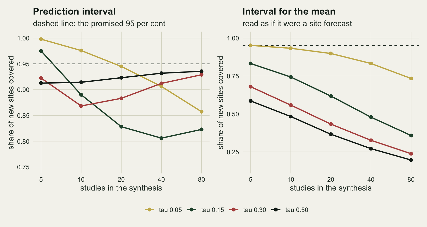
A between-site variance that is often exactly zero
The prediction interval stands on the estimate of tau-squared. The moment estimator is truncated at zero, and when it lands there the prediction interval collapses onto the confidence interval for the mean with a t multiplier, which the right panel above has shown (with a z multiplier) to be a poor forecast.
z_at <- function(k, tau) cv(k, tau, "dl_t", "zero")
cc_k40 <- runs[[which(cells$k == 40 & cells$tau == 0.15)]]$cc_dl_t
b90_k40 <- mean(cc_k40 < 0.90); b80_k40 <- mean(cc_k40 < 0.80)
med_k40 <- median(cc_k40)
zf_k40 <- runs[[which(cells$k == 40 & cells$tau == 0.15)]]$zero_dl
zero_in_b80 <- mean(zf_k40[cc_k40 < 0.80])
b90_k5 <- cv(5, 0.15, "dl_t", "below90")
cz_k40 <- cv(40, 0.15, "dl_t", "cc_zero")
The share of syntheses with an estimate of exactly zero is 0.59 at five studies and tau 0.05, and more studies bring it down only to 0.49 at eighty. At tau 0.15 it falls from 0.48 at five studies to 0.23 at forty and 0.12 at eighty. At tau 0.5 it is 0.11 at five studies and at most 0.002 from twenty studies on.
That explains the shape of the left panel above. With five studies a zero estimate is common, but the t quantile on three degrees of freedom is 3.18, and an interval that wide covers a small spread of site effects whatever tau-squared does. By forty studies the quantile has fallen to 2.02, the standard error of the mean has shrunk, and the syntheses that returned zero now report an interval that is too narrow for the sites. Coverage is lowest where the multiplier has stopped compensating and tau-squared has not yet become estimable.
The average also hides a spread. A synthesis is one draw, and the reader of it gets the coverage of that one interval, not the average. At forty studies and tau 0.15 the median synthesis reports an interval that covers 0.934 of sites, so a typical interval looks fine, but 0.44 of the syntheses cover less than 90 per cent and 0.34 less than 80 per cent. The average of 0.806 is a mixture of intervals near nominal and intervals far below it, and the right panel below shows the two groups. The clump near 0.45 is the syntheses that returned a zero: on average their intervals cover 0.444 of new sites. Of the syntheses below 80 per cent, 0.68 returned a zero; the others fill the flat stretch between the two groups. At five studies the share below 90 per cent is 0.07.
z_tab <- dlt
z_tab$tau_f <- factor(sprintf("tau %.2f", z_tab$tau), levels = tau_lab)
p_zero <- ggplot(z_tab, aes(k, zero, colour = tau_f)) +
  geom_line(linewidth = 0.9) + geom_point(size = 2) +
  scale_x_log10(breaks = k_grid) +
  scale_colour_manual(values = tau_cols, name = NULL) +
  scale_y_continuous(limits = c(0, 1)) +
  labs(x = "studies in the synthesis", y = "share with tau-squared at zero",
       title = "Estimates on the boundary", subtitle = "DerSimonian-Laird, truncated at zero") +
  theme_datasheet() + theme(legend.position = "bottom")
p_hist <- ggplot(data.frame(cc = cc_k40), aes(cc)) +
  geom_histogram(breaks = seq(0.3, 1, by = 0.02), fill = te_forest, colour = te_paper, linewidth = 0.2) +
  geom_vline(xintercept = 0.95, colour = te_rust, linetype = "dashed", linewidth = 0.8) +
  labs(x = "share of new sites this synthesis covers", y = "syntheses",
       title = "One interval per synthesis", subtitle = "forty studies, tau 0.15; dashed line: 95 per cent") +
  theme_datasheet()
p_zero + p_hist + plot_annotation(theme = theme_datasheet())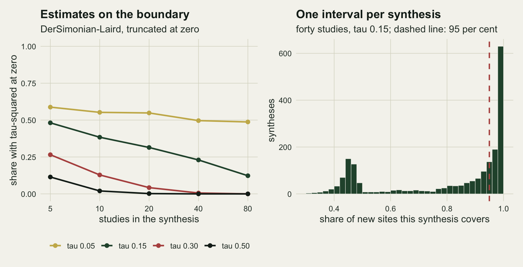
More studies do not rescue the smallest spread. The grid stopped at eighty studies, so one chunk pushes two cells to 320, and compares three ways of making the studies at tau 0.15: g from simulated arms as above, the same g with its variance computed at the true mean instead of at g itself, and normal effects whose variance is known exactly, the textbook model the interval is derived under.
set.seed(6340)
ext_cell <- function(k, tau, generator) {
  s <- sim_syntheses(n_rep, k, tau, generator)
  t2 <- tau2_dl(s$g, s$v); f_e <- pool(s$g, s$v, t2)
  h_e <- qt(0.975, k - 2) * sqrt(t2 + f_e$se^2)
  c(coverage = mean(cond_cover(f_e$m - h_e, f_e$m + h_e, tau)), zero = mean(t2 == 0),
    bias_mean = mean(f_e$m) - mu_true)
}
ext_05 <- ext_cell(320, 0.05, "arms")
ext_15 <- sapply(c(arms = "arms", arms_mu = "arms_mu", normal = "normal"),
                 function(gn) ext_cell(320, 0.15, gn))
At tau 0.05 and 320 studies coverage is 0.707, with 0.48 of the estimates still exactly zero: a between-site standard deviation of 0.05 against within-study standard errors between 0.22 and 0.50 is not estimable at any number of studies a synthesis in ecology will see. At tau 0.15 coverage does recover by 320 studies, to 0.924 for the textbook model and 0.899 for g from arms. The shortfall of the arms comes from plugging g into its own variance, which ties each study’s weight to its effect and pulls the pooled mean off by -0.0064: with the variance computed at the true mean the same effects reach 0.935, and the mean is off by -0.0001.
Changing the estimator does not fix it
If the trouble is a tau-squared estimate that sits on zero, a better estimator is the obvious first move. Veroniki and colleagues 2016 review the options and recommend REML or Paule-Mandel over DerSimonian-Laird for most purposes. Both were scored on the same syntheses above. Two further repairs aim at the uncertainty in tau-squared rather than its point value. One plugs the upper end of the Q-profile interval for tau-squared (Viechtbauer 2007), the same uniroot inversion the heterogeneity post uses, into the prediction interval. The other is a parametric bootstrap of the studentised distance between a new site’s effect and the pooled mean, which lets the data set the multiplier instead of the t distribution. The bootstrap is slower, so it is run on fewer syntheses and only at tau 0.15.
n_boot_syn <- 1000; n_boot <- 200; k_boot <- c(5, 10, 20, 40); tau_boot <- 0.15
boot_cell <- function(k, tau, block = 50) {
  s <- sim_syntheses(n_boot_syn, k, tau); g <- s$g; v <- s$v
  t2 <- tau2_dl(g, v); f_hat <- pool(g, v, t2); scl <- sqrt(t2 + f_hat$se^2)
  lo_i <- hi_i <- numeric(n_boot_syn)
  for (st in seq(1, n_boot_syn, by = block)) {
    idx <- st:min(n_boot_syn, st + block - 1); nb <- length(idx) * n_boot
    vb <- v[rep(idx, each = n_boot), , drop = FALSE]
    mb <- rep(f_hat$m[idx], each = n_boot); tb <- rep(t2[idx], each = n_boot)
    gb <- matrix(rnorm(nb * k, mb, sqrt(vb + tb)), nb, k)
    t2b <- tau2_dl(gb, vb); fb <- pool(gb, vb, t2b)
    pivot <- (rnorm(nb, mb, sqrt(tb)) - fb$m) / sqrt(t2b + fb$se^2)
    qs <- apply(matrix(pivot, length(idx), n_boot, byrow = TRUE), 1, quantile, c(0.025, 0.975))
    lo_i[idx] <- f_hat$m[idx] + qs[1, ] * scl[idx]
    hi_i[idx] <- f_hat$m[idx] + qs[2, ] * scl[idx]
  }
  cc_b <- cond_cover(lo_i, hi_i, tau)
  data.frame(k = k, tau = tau, interval = "boot", coverage = mean(cc_b),
             mcse = sd(cc_b) / sqrt(n_boot_syn), width = mean(hi_i - lo_i),
             cover_zero = mean(cc_b[t2 == 0]))
}
set.seed(5120)
boot_tab <- do.call(rbind, lapply(k_boot, boot_cell, tau = tau_boot))
bt <- function(k, col = "coverage") boot_tab[boot_tab$k == k, col]
pm_gap   <- max(abs(grid_tab$coverage[grid_tab$interval == "pm_t"] - dlt$coverage))
reml_gap <- max(abs(grid_tab$coverage[grid_tab$interval == "reml_t"] - dlt$coverage))
zero_gap <- max(abs(grid_tab$zero_reml - grid_tab$zero))
qp_min   <- min(grid_tab$coverage[grid_tab$interval == "qp_t"])
w_ratio  <- function(k, tau) cv(k, tau, "qp_t", "width") / cv(k, tau, "dl_t", "width")
Neither estimator moves the numbers. Across all twenty cells, Paule-Mandel coverage differs from DerSimonian-Laird coverage by at most 0.008 and REML by at most 0.008, and the share of zero estimates under REML differs from the moment estimator’s by at most 0.031. A different point estimate of a quantity that the data cannot pin down lands on the same boundary.
The bootstrap does not repair it either. At tau 0.15 its coverage is 0.847, 0.812, 0.806 and 0.832 at five, ten, twenty and forty studies, against 0.975, 0.890, 0.828 and 0.806 for the t interval. It gives up the conservatism of the t multiplier at five studies, is lower than the t interval at ten and twenty, and is 0.026 higher at forty, where its Monte Carlo standard error is 0.008. The reason is the same boundary: a synthesis with a zero estimate is resampled from a world with no between-site spread, and in that world the bootstrap learns that none is needed. Among those syntheses the bootstrap interval covers 0.368 of sites at forty studies.
The Q-profile upper bound does what it promises and more. Its lowest coverage anywhere in the grid is 0.983. The price is width: at forty studies and tau 0.15 the interval is 2.2 times as wide as the t interval, and at ten studies 3.1 times. It answers a different question, how far a new site could plausibly be if the spread among sites is as large as the data allow, and for a manager deciding whether an intervention is worth trying it is a legitimate second number, not a replacement.
iv_lab <- c(dl_t = "DerSimonian-Laird, t", reml_t = "REML, t", dl_z = "DerSimonian-Laird, z",
            qp_t = "Q-profile upper tau, t", boot = "parametric bootstrap")
est_tab <- rbind(grid_tab[grid_tab$tau == 0.15 & grid_tab$interval %in% c("dl_t", "reml_t", "dl_z", "qp_t"),
                          c("k", "interval", "coverage", "width")],
                 boot_tab[, c("k", "interval", "coverage", "width")])
est_tab$iv <- factor(iv_lab[est_tab$interval], levels = iv_lab)
iv_cols <- c(te_forest, te_gold, te_body, te_rust, te_ink)
iv_lty  <- c("solid", "dashed", "dotted", "solid", "solid")
p_est_c <- ggplot(est_tab, aes(k, coverage, colour = iv, linetype = iv)) +
  geom_hline(yintercept = 0.95, colour = te_line, linewidth = 1.2) +
  geom_line(linewidth = 0.9) + geom_point(size = 1.8) +
  scale_x_log10(breaks = k_grid) +
  scale_colour_manual(values = iv_cols, name = NULL) +
  scale_linetype_manual(values = iv_lty, name = NULL) +
  guides(colour = guide_legend(nrow = 2), linetype = guide_legend(nrow = 2)) +
  labs(x = "studies in the synthesis", y = "share of new sites covered",
       title = "Coverage", subtitle = "thick pale line: 95 per cent") +
  theme_datasheet()
p_est_w <- ggplot(est_tab, aes(k, width, colour = iv, linetype = iv)) +
  geom_line(linewidth = 0.9) + geom_point(size = 1.8) +
  geom_hline(yintercept = 2 * qnorm(0.975) * 0.15, colour = te_body, linetype = "dashed", linewidth = 0.4) +
  scale_x_log10(breaks = k_grid) + scale_y_log10() +
  scale_colour_manual(values = iv_cols, name = NULL) +
  scale_linetype_manual(values = iv_lty, name = NULL) +
  guides(colour = guide_legend(nrow = 2), linetype = guide_legend(nrow = 2)) +
  labs(x = "studies in the synthesis", y = "mean interval width (log scale)",
       title = "Width", subtitle = "dashed line: width if tau were known") +
  theme_datasheet()
p_est_c + p_est_w + plot_layout(guides = "collect") +
  plot_annotation(theme = theme_datasheet() + theme(legend.position = "bottom"))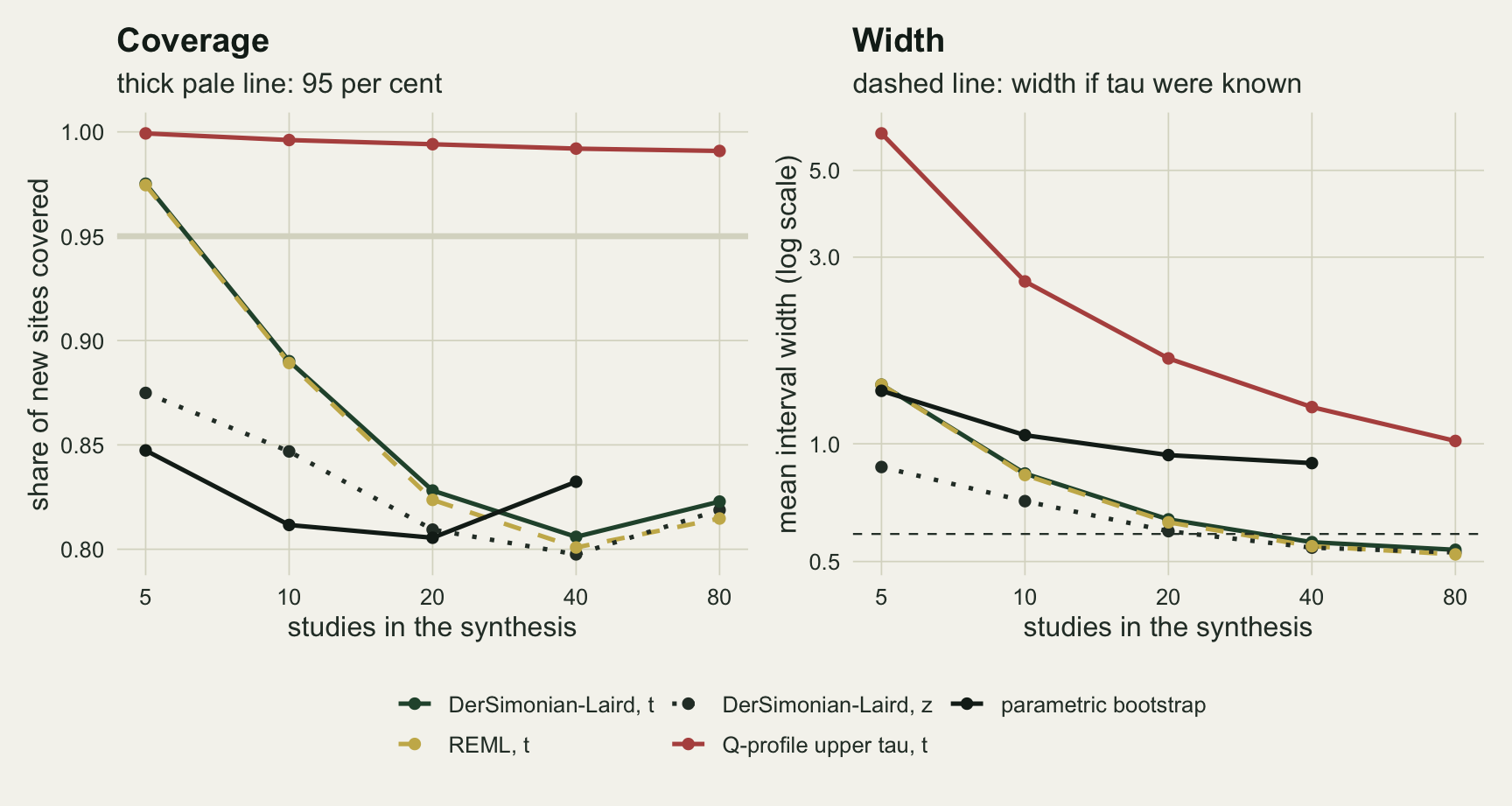
An observed replicate at a new site
The manager will not observe her site’s true effect. She will run one exclosure experiment and get an estimate with its own sampling error, and the question becomes whether that estimate is consistent with the synthesis. The interval for an observed replicate adds the replicate’s sampling variance to the prediction variance. That variance is known from the replicate’s sample size, so it does not need estimating, and when it is large next to tau-squared the part of the interval that is badly estimated is a small share of the total.
n_new <- 20                                  # plots per arm at the new site
set.seed(7231)
rep_tab <- do.call(rbind, lapply(c(0.05, 0.15), function(tt) do.call(rbind, lapply(k_grid, function(kk) {
  s <- sim_syntheses(n_rep, kk, tt)
  t2 <- tau2_dl(s$g, s$v); f_r <- pool(s$g, s$v, t2); crit <- qt(0.975, kk - 2)
  y_site <- draw_g(rnorm(n_rep, mu_true, tt), rep(n_new, n_rep))
  v_site <- 2 / n_new + f_r$m^2 / (4 * n_new)
  h_true <- crit * sqrt(t2 + f_r$se^2); h_obs <- crit * sqrt(t2 + f_r$se^2 + v_site)
  data.frame(k = kk, tau = tt,
             target = c("true effect at the site", "observed replicate at the site"),
             coverage = c(mean(cond_cover(f_r$m - h_true, f_r$m + h_true, tt)),
                          mean(abs(y_site - f_r$m) <= h_obs)))
}))))
rp <- function(k, tau, tg) rep_tab$coverage[rep_tab$k == k & rep_tab$tau == tau & grepl(tg, rep_tab$target)]
mcse_rep <- sqrt(0.95 * 0.05 / n_rep)
rep_min  <- min(rep_tab$coverage[grepl("observed", rep_tab$target)])
true_min <- min(rep_tab$coverage[grepl("true", rep_tab$target)])
With 20 plots per arm at the new site, the interval for the observed replicate covers 0.953 of replicates at forty studies and tau 0.15, where the interval for the true effect covered 0.805. At tau 0.05 and eighty studies the two are 0.947 and 0.838. The binomial Monte Carlo standard error of the replicate rates is about 0.0049. Across the ten cells the replicate interval never covers less than 0.936, against a lowest 0.805 for the true effect, although at five studies both are conservative and the replicate interval more so, because its t multiplier on three degrees of freedom also inflates the replicate’s sampling variance, which is known and needs no such allowance. So the target matters: a synthesis that cannot predict a site’s true effect can still be close to honest about what one experiment at that site will return, because most of that uncertainty is sampling error it knows how to compute. The replicate interval is not immune; it slips to 0.936 at eighty studies and tau 0.15, as the prediction part of it narrows.
The same idea underlies the replication interval of Patil, Peng and Leek 2016, which asks whether a replicate falls inside an interval built from one original study and the two sampling variances. Their interval has no tau-squared in it, and a new site is not the original site. The last chunk adds two tau-squared to it, one for each site, uses the true tau as the most favourable case, and scores it with and without a significance filter on the original, because originals that get replicated are usually the ones that were significant.
n_orig <- 10; tau_rep <- 0.2; n_single <- 20000; z975 <- qnorm(0.975)
set.seed(8802)
patil_cell <- function(mu_o, filter_sig) {
  s_o <- sqrt(2 / n_orig)
  y_o <- rnorm(n_single, rnorm(n_single, mu_o, tau_rep), s_o)
  y_r <- rnorm(n_single, rnorm(n_single, mu_o, tau_rep), s_o)
  keep <- if (filter_sig) y_o / s_o > z975 else rep(TRUE, n_single)
  c(without_tau = mean(abs(y_r - y_o)[keep] <= z975 * sqrt(2 * s_o^2)),
    with_tau    = mean(abs(y_r - y_o)[keep] <= z975 * sqrt(2 * s_o^2 + 2 * tau_rep^2)),
    kept = sum(keep))
}
patil_tab <- rbind(all_03 = patil_cell(mu_true, FALSE), sig_03 = patil_cell(mu_true, TRUE),
                   sig_00 = patil_cell(0, TRUE))
patil_closed <- 2 * pnorm(z975 * sqrt((4 / n_orig) / (4 / n_orig + 2 * tau_rep^2))) - 1
With 10 plots per arm and tau 0.2, the interval without tau accepts 0.928 of replicates of unselected originals, and the closed form gives 0.926; adding two tau-squared brings it to 0.950. With a significance filter on the original the acceptance rates fall, to 0.792 and 0.846, because a significant original from ten plots per arm overstates its effect, the winner’s curse described in Power analysis by simulation in R. When the true mean is zero and only the 710 significant originals out of 20000 are replicated, the interval without tau accepts 0.655 of the replicates and the interval with tau 0.734. The term that makes the interval honest for a new site also makes it more willing to call a replication of an original whose mean effect is zero a success. That is not a reason to leave tau out; it is a reason not to read “inside the prediction interval” as confirmation.
r15 <- rep_tab[rep_tab$tau == 0.15, ]
r15$target <- factor(r15$target, levels = c("true effect at the site", "observed replicate at the site"))
p_rep <- ggplot(r15, aes(k, coverage, colour = target)) +
  geom_hline(yintercept = 0.95, colour = te_body, linetype = "dashed", linewidth = 0.5) +
  geom_line(linewidth = 0.9) + geom_point(size = 2) +
  scale_x_log10(breaks = k_grid) +
  scale_colour_manual(values = c(te_forest, te_gold), name = NULL) +
  coord_cartesian(ylim = c(0.75, 1)) +
  guides(colour = guide_legend(nrow = 2)) +
  labs(x = "studies in the synthesis", y = "share covered",
       title = "What is being predicted", subtitle = "tau 0.15, twenty plots per arm at the new site") +
  theme_datasheet() + theme(legend.position = "bottom")
pat_long <- data.frame(
  case = factor(rep(c("all,\nmean 0.3", "significant,\nmean 0.3",
                      "significant,\nmean 0"), each = 2),
                levels = c("all,\nmean 0.3", "significant,\nmean 0.3",
                           "significant,\nmean 0")),
  version = factor(rep(c("without tau", "with two tau-squared"), 3),
                   levels = c("without tau", "with two tau-squared")),
  rate = c(t(patil_tab[, c("without_tau", "with_tau")])))
p_pat <- ggplot(pat_long, aes(case, rate, fill = version)) +
  geom_col(position = position_dodge(width = 0.75), width = 0.65, colour = te_paper, linewidth = 0.3) +
  geom_hline(yintercept = 0.95, colour = te_body, linetype = "dashed", linewidth = 0.5) +
  scale_fill_manual(values = c(te_rust, te_forest), name = NULL) +
  scale_y_continuous(limits = c(0, 1)) +
  guides(fill = guide_legend(nrow = 2)) +
  labs(x = NULL, y = "replicates inside the interval",
       title = "One original, one replicate", subtitle = "ten plots per arm, tau 0.2") +
  theme_datasheet() + theme(legend.position = "bottom")
p_rep + p_pat + plot_annotation(theme = theme_datasheet())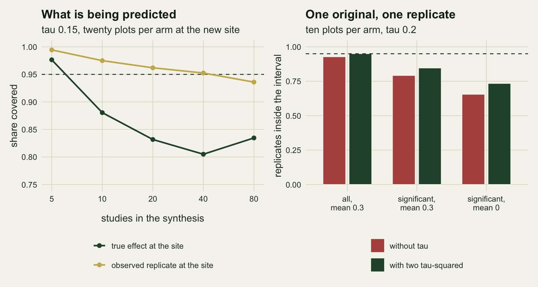
What to report
Report the prediction interval, and report the number of studies and the estimate of tau-squared next to it, including when that estimate is zero. A zero is the most informative thing a reader can be told about the interval: it means the prediction interval is the confidence interval for the mean with a wider multiplier, and at twenty or more studies that is an interval for the mean, not for a site.
Report the upper end of the Q-profile interval for tau-squared, and the prediction interval it implies, as a second number. It is too wide to serve as the headline, but it states what the synthesis cannot rule out about the next site, which is the question the manager asked.
Do not switch estimators to rescue the interval. REML and Paule-Mandel are defensible choices for tau-squared on other grounds, but in this simulation they left the coverage of the prediction interval where DerSimonian-Laird put it.
If the practical question is what one experiment at a new site will return, say so and build the interval for an observed replicate, with the replicate’s sampling variance added. In the cells measured here it never fell far below its nominal coverage while the interval for the true effect did, and it is the interval a follow-up study can actually be checked against. When a single original is used instead of a synthesis, include between-site variance in the replication interval and do not treat a replicate falling inside it as evidence that the original effect was real.
Honest limits
The between-site effects are normal, and the whole simulation is on one effect-size scale, Hedges g with 8 to 40 plots per arm and a mean of 0.3. Skewed or heavy-tailed site effects were not simulated. The log response ratio case in Meta-analysis of little-replicated experiments shows effect sizes whose variances are themselves poorly estimated, which this post does not cover. The mean of 0.3 matters too, because the variance formula for g depends on g; a mean of zero would weaken the weight-effect link measured at 320 studies.
Every study in a synthesis is independent and unbiased. Real syntheses carry several effects per study and a filtered literature, and a prediction interval inherits every bias of the mean it is centred on.
Coverage was scored against the distribution the studies were drawn from. A manager’s site is not a random draw from the sites that were studied; a degraded meadow chosen because it is degraded may sit in the tail. No interval computed from the synthesis can fix that, and the numbers above are the best case for it.
The bootstrap tried here is one construction, a parametric resampling of a studentised pivot from the DerSimonian-Laird fit, with 200 resamples and 1000 syntheses per cell. Other published bootstrap and Bayesian predictive intervals propagate the uncertainty in tau-squared differently and may do better; a Bayesian interval with an informative prior on tau is the natural candidate when there are few studies, and it was not tested.
The replication section uses the true tau in the single-original interval. In practice tau has to come from somewhere else, usually a synthesis of related studies, and all the estimation trouble of the earlier sections comes with it.
References
DerSimonian R, Laird N 1986 Controlled Clinical Trials 7(3):177-188 (10.1016/0197-2456(86)90046-2)
Higgins JPT, Thompson SG, Spiegelhalter DJ 2009 Journal of the Royal Statistical Society Series A 172(1):137-159 (10.1111/j.1467-985X.2008.00552.x)
IntHout J, Ioannidis JPA, Rovers MM, Goeman JJ 2016 BMJ Open 6(7):e010247 (10.1136/bmjopen-2015-010247)
Partlett C, Riley RD 2017 Statistics in Medicine 36(2):301-317 (10.1002/sim.7140)
Veroniki AA, Jackson D, Viechtbauer W, Bender R, Bowden J, Knapp G, Kuss O, Higgins JPT, Langan D, Salanti G 2016 Research Synthesis Methods 7(1):55-79 (10.1002/jrsm.1164)
Viechtbauer W 2007 Statistics in Medicine 26(1):37-52 (10.1002/sim.2514)
Patil P, Peng RD, Leek JT 2016 Perspectives on Psychological Science 11(4):539-544 (10.1177/1745691616646366)