library(ggplot2)
library(patchwork)
library(mgcv)

te_paper  <- "#f5f4ee"
te_ink    <- "#16241d"
te_body   <- "#2c3a31"
te_forest <- "#275139"
te_rust   <- "#b5534e"
te_gold   <- "#c9b458"
te_line   <- "#dad9ca"

theme_datasheet <- function() {
  theme_minimal(base_size = 12) +
    theme(plot.background  = element_rect(fill = te_paper, colour = NA),
          panel.background = element_rect(fill = te_paper, colour = NA),
          panel.grid.major = element_line(colour = te_line, linewidth = 0.3),
          panel.grid.minor = element_blank(),
          text             = element_text(colour = te_body),
          plot.title       = element_text(colour = te_ink, face = "bold"),
          plot.subtitle    = element_text(colour = te_body),
          axis.text        = element_text(colour = te_body))
}Novel climate combinations and the MESS map
R
species distribution models
climate change
collinearity
GAMs
mgcv
simulation
ecology tutorial
When temperature and rainfall are correlated, a warmer and wetter future passes a one-covariate MESS check yet leaves the data. Measuring the damage in mgcv.
A shrub grows across a region where the warm lowlands are also the dry lowlands. Its occupancy has been surveyed at a few hundred sites, and a binomial GAM with a smooth of temperature and a smooth of precipitation fits them well. The climate scenario for the end of the century is warmer and wetter, and the map of projected occupancy is the deliverable. Before handing it over, the analyst runs the novelty check this site teaches: for each future cell, is every covariate inside the range it had in the survey? Most cells are, and the map goes out.
The check asked the wrong question. In this region temperature and precipitation are strongly negatively correlated, so the survey sampled a narrow strip of the climate plane running from cool and wet to warm and dry. A future that is warmer and wetter moves the cells across that strip rather than along it. Each covariate on its own can stay inside its sampled range while the pair lands in a combination that no surveyed site ever had. Williams and Jackson called such futures novel climates, and the problem is well known in the distribution modelling literature. Dormann and colleagues showed by simulation in 2013 that prediction degrades when the collinearity structure of the new data differs from the training data, and Mesgaran, Cousens and Webber defined in 2014 a second novelty measure, NT2, for exactly this kind of change: a Mahalanobis distance from the training data, scaled by the largest such distance inside it, which sits beside the one-covariate range check. This post is a demonstration of those published results, not a claim to them. What it measures is narrower: how much more widely the projection scatters across the correlation than along it, for a model that is correctly specified as well as for two that are not; what share of the future cells the one-covariate check passes while NT2 flags them; which way the additive model’s bias points, and why; and what a small decoupled sample buys.
The neighbours on this site set the scene from two sides. Collinearity and VIF in ecological regression states up front that collinearity “does not hurt prediction”, and backs it with the agreement of two models’ fitted values on the data they were fitted to. That is true in the sample. The projections below leave the sample in the one direction the correlation never covered. Checking a presence-only model builds the multivariate environmental similarity surface of Elith, Kearney and Phillips, the MESS, scoring each covariate by its distance from the nearer edge of the training range and taking the minimum; its example has one covariate running past its band, which the MESS sees. Here the failing cells pass that test. SDM fitted before the invasion is over notes in its limits that a Mahalanobis-type distance in a correlated set behaves differently from degrees on one axis; this post measures that difference on one design.
A region where warm means dry
n_cell     <- 3000
n_site     <- 300
n_off      <- 30
sd_scatter <- 0.10
a_shift    <- 0.2
n_draw     <- 20
n_extra    <- 10

make_cells <- function(n) {
  temp <- runif(n)
  data.frame(temp = temp,
             prec = pmin(pmax(1 - temp + rnorm(n, 0, sd_scatter), 0), 1))
}
shifts <- list(along = c(a_shift, -a_shift), across = c(a_shift, a_shift))
shift_cells <- function(cells, s) data.frame(temp = cells$temp + s[1],
                                             prec = cells$prec + s[2])

truths <- list(
  threshold = function(temp, prec) 2 - 10 * pmax(0, temp - prec + 0.1),
  unimodal  = function(temp, prec) 2 - 8 * (temp - prec)^2,
  linear    = function(temp, prec) 0.5 - 3 * (temp - prec),
  convex    = function(temp, prec) -3 + 10 * pmax(0, temp - prec - 0.1),
  weak      = function(temp, prec) 2 - 3 * pmax(0, temp - prec + 0.1))
main_truths <- c("threshold", "unimodal", "linear")
truth_lab <- c(threshold = "threshold", unimodal = "unimodal", linear = "linear",
               convex = "convex", weak = "weak threshold")

draw_world <- function(k) {
  set.seed(4400 + k)
  cells    <- make_cells(n_cell)
  idx      <- sample.int(n_cell, n_site)
  district <- data.frame(temp = runif(n_off), prec = runif(n_off))
  list(cells = cells, idx = idx, district = district,
       u_site = runif(n_site), u_dist = runif(n_off))
}

set.seed(4400)
big_cells <- make_cells(1e5)
r_tp <- cor(big_cells$temp, big_cells$prec)
sd_deficit <- sd(big_cells$temp - big_cells$prec)
sd_sum     <- sd(big_cells$temp + big_cells$prec)
The region has 3000 grid cells. Temperature and precipitation are both scaled to run from 0 to 1; temperature is uniform, and precipitation is one minus temperature plus normal scatter with a standard deviation of 0.10, clipped to the unit interval. The correlation between them is -0.95. Each simulated survey visits 300 cells at random and records presence or absence, drawn from the cell’s true probability of occupancy.
A useful pair of coordinates is the deficit, temperature minus precipitation, a crude water balance, and the sum, temperature plus precipitation. In this region the deficit has a standard deviation of 0.577 across cells and the sum only 0.095: the data are a long strip along the deficit and a thin one across it. The two futures are shifts of the same length. Along the strip, warmer by 0.2 and drier by 0.2, the deficit rises by 0.4 and the sum stays put. Across the strip, warmer by 0.2 and wetter by 0.2, the sum rises by 0.4, four times the scatter that is the only information the survey has in that direction, and the deficit stays put.
Five true responses are used, all written on the logit scale and all functions of the deficit alone. The threshold species is fine until the deficit passes -0.1 and then declines steeply, at 10 logit units per unit of deficit; the weak threshold has the same kink with a slope of 3; the convex species is the mirror image, favoured by dry conditions past a deficit of 0.1; the unimodal species has an optimum at a deficit of zero, a quadratic on the logit scale; and the linear species declines steadily with the deficit. The linear truth is the control, because a model that is additive in temperature and precipitation is exactly right for it: 0.5 - 3 (T - P) is a straight line in T plus a straight line in P. Since every truth depends on the deficit alone and the across shift does not change the deficit, the true change in occupancy under the warmer and wetter future is exactly zero for all five species. The along shift has a real, negative effect for four of them and a positive one for the convex species.
What the MESS map sees
mess_strip <- function(fut, train) {
  nov <- function(v, x) pmin(v - min(x), max(x) - v)
  pmin(nov(fut$temp, train$temp), nov(fut$prec, train$prec))
}
mess_full <- function(fut, train) {
  one_cov <- function(v, x) {
    f_pct <- 100 * ecdf(x)(v) - 100 * (v %in% x) / length(x)
    lo <- min(x); hi <- max(x)
    ifelse(v < lo, 100 * (v - lo) / (hi - lo),
      ifelse(v > hi, 100 * (hi - v) / (hi - lo),
        ifelse(f_pct <= 50, 2 * f_pct, 2 * (100 - f_pct))))
  }
  pmin(one_cov(fut$temp, train$temp), one_cov(fut$prec, train$prec))
}
nt2_parts <- function(fut, train) {
  mu <- colMeans(train); s_mat <- cov(train)
  d_train <- sqrt(mahalanobis(train, mu, s_mat))
  list(d_fut = sqrt(mahalanobis(fut, mu, s_mat)),
       d_max = max(d_train), d_q99 = unname(quantile(d_train, 0.99)))
}
geo_one <- function(train, cells) {
  out <- c()
  for (nm in names(shifts)) {
    fut    <- shift_cells(cells, shifts[[nm]])
    inside <- mess_strip(fut, train) >= 0
    nt     <- nt2_parts(fut, train)
    out_max <- nt$d_fut / nt$d_max > 1
    out_q99 <- nt$d_fut / nt$d_q99 > 1
    out <- c(out, setNames(c(mean(inside), mean(out_max), mean(inside & out_max),
                             mean(out_q99), mean(inside & out_q99)),
                           paste(nm, c("mess_in", "nt2_out", "blind",
                                       "q99_out", "blind_q99"), sep = "_")))
  }
  out
}

geo_rows <- list()
full_check <- list()
dist_check <- list()
for (k in seq_len(n_draw)) {
  w <- draw_world(k)
  train0  <- w$cells[w$idx, ]
  train30 <- rbind(w$cells[w$idx[seq_len(n_site - n_off)], ], w$district)
  geo_rows[[length(geo_rows) + 1]] <- data.frame(draw = k, arm = 0, t(geo_one(train0, w$cells)))
  geo_rows[[length(geo_rows) + 1]] <- data.frame(draw = k, arm = 30, t(geo_one(train30, w$cells)))
  fut_ac <- shift_cells(w$cells, shifts$across)
  ms <- mess_strip(fut_ac, train0); mf <- mess_full(fut_ac, train0)
  nt <- nt2_parts(fut_ac, train0)
  blind <- ms >= 0 & nt$d_fut > nt$d_max
  fut_al <- shift_cells(w$cells, shifts$along)
  mf_al <- mess_full(fut_al, train0)
  full_check[[k]] <- c(sign_disagree = mean((ms >= 0) != (mf >= 0)),
                       blind_full_med = median(mf[blind]),
                       along_in_full_med = median(mf_al[mess_strip(fut_al, train0) >= 0]),
                       ratio_max_q99 = nt$d_max / nt$d_q99)
  # with the district: which site sets the maximum, and the strip sites' own maximum
  d30 <- sqrt(mahalanobis(train30, colMeans(train30), cov(train30)))
  d30_fut <- sqrt(mahalanobis(fut_ac, colMeans(train30), cov(train30)))
  strip_max <- max(d30[seq_len(n_site - n_off)])
  dist_check[[k]] <- c(max_is_district = unname(which.max(d30)) > n_site - n_off,
                       d_max = max(d30), d_max_strip = strip_max,
                       out_strip = mean(d30_fut > strip_max),
                       blind_strip = mean(mess_strip(fut_ac, train30) >= 0 & d30_fut > strip_max))
}
geo <- do.call(rbind, geo_rows)
full_check <- do.call(rbind, full_check)
dist_check <- do.call(rbind, dist_check)
g0  <- geo[geo$arm == 0, ]
g30 <- geo[geo$arm == 30, ]
q3  <- function(x) c(med = median(x), lo = min(x), hi = max(x))
blind_q  <- q3(g0$across_blind)
nt2_q    <- q3(g0$across_nt2_out)
q99_q    <- q3(g0$across_q99_out)
blindq99 <- q3(g0$across_blind_q99)
The MESS used here is the one from the presence-only check, without the percentile refinement: for each covariate, the distance of the future value from the nearer edge of the surveyed range, and the minimum over the two covariates. A cell is inside when that minimum is at least zero. NT2 is the Mahalanobis distance of the future cell from the centre of the surveyed sites, using their covariance matrix, divided by the largest such distance among the surveyed sites themselves; a value above one means the cell is farther from the data, in the metric the correlation defines, than any site that was visited.
Over the 20 surveys, the MESS calls 0.757 of the along future cells inside (median over surveys) and 0.601 of the across future cells. The difference comes from the ends of the strip: a shift of 0.2 pushes the warmest cells past the warmest site in both futures, and the across shift also pushes the wettest cells past the wettest site. NT2 tells the two futures apart. Along the strip it flags 0.006 of the cells. Across it flags 0.893, ranging from 0.728 to 0.961 over surveys.
The share that matters is the overlap: future cells inside every single-covariate range that NT2 puts outside anything sampled. Across the strip it is 0.502, from 0.362 to 0.564. The denominator is all 3000 future cells of one survey; the median and range are over surveys. These shares are geometry, fixed by the two grids and the shift, not a property of any fitted model, and they are the same whichever species is being modelled.
w1 <- draw_world(1)
tr1 <- w1$cells[w1$idx, ]
nt1_mu <- colMeans(tr1); nt1_s <- cov(tr1)
nt1_max <- max(sqrt(mahalanobis(tr1, nt1_mu, nt1_s)))
plane <- expand.grid(temp = seq(-0.1, 1.3, length.out = 241),
                     prec = seq(-0.1, 1.3, length.out = 241))
plane$d_rel <- sqrt(mahalanobis(plane[, c("temp", "prec")], nt1_mu, nt1_s)) / nt1_max
class_cells <- function(nm) {
  fut <- shift_cells(w1$cells, shifts[[nm]])
  ins <- mess_strip(fut, tr1) >= 0
  outj <- sqrt(mahalanobis(fut, nt1_mu, nt1_s)) / nt1_max > 1
  fut$class <- ifelse(!ins, "outside a single range",
                      ifelse(outj, "inside every range, outside joint",
                             "inside every range and joint"))
  fut$future <- paste0(nm, ": warmer by 0.2, ",
                       ifelse(nm == "along", "drier by 0.2", "wetter by 0.2"))
  fut
}
geo_df <- rbind(class_cells("along"), class_cells("across"))
geo_df$future <- factor(geo_df$future, levels = unique(geo_df$future))
geo_df$class <- factor(geo_df$class, levels = c("inside every range and joint",
                                                "inside every range, outside joint",
                                                "outside a single range"))
box_df <- data.frame(xmin = min(tr1$temp), xmax = max(tr1$temp),
                     ymin = min(tr1$prec), ymax = max(tr1$prec))
ggplot(geo_df, aes(temp, prec)) +
  geom_point(aes(colour = class), size = 0.45, alpha = 0.6) +
  geom_rect(data = box_df, aes(xmin = xmin, xmax = xmax, ymin = ymin, ymax = ymax),
            inherit.aes = FALSE, fill = NA, colour = te_body, linetype = "dashed",
            linewidth = 0.5) +
  geom_contour(data = plane, aes(z = d_rel), breaks = 1, colour = te_ink,
               linewidth = 0.6) +
  geom_point(data = tr1, colour = te_ink, size = 0.5) +
  facet_wrap(~future) +
  coord_equal(xlim = c(-0.05, 1.25), ylim = c(-0.05, 1.25)) +
  scale_colour_manual(values = c(te_forest, te_rust, te_gold), name = NULL) +
  guides(colour = guide_legend(override.aes = list(size = 2.5, alpha = 1))) +
  labs(x = "temperature (scaled)", y = "precipitation (scaled)",
       title = "Inside every range, outside the data",
       subtitle = "black: surveyed sites; dashed box: their ranges; solid lines: NT2 = 1") +
  theme_datasheet() +
  theme(legend.position = "bottom")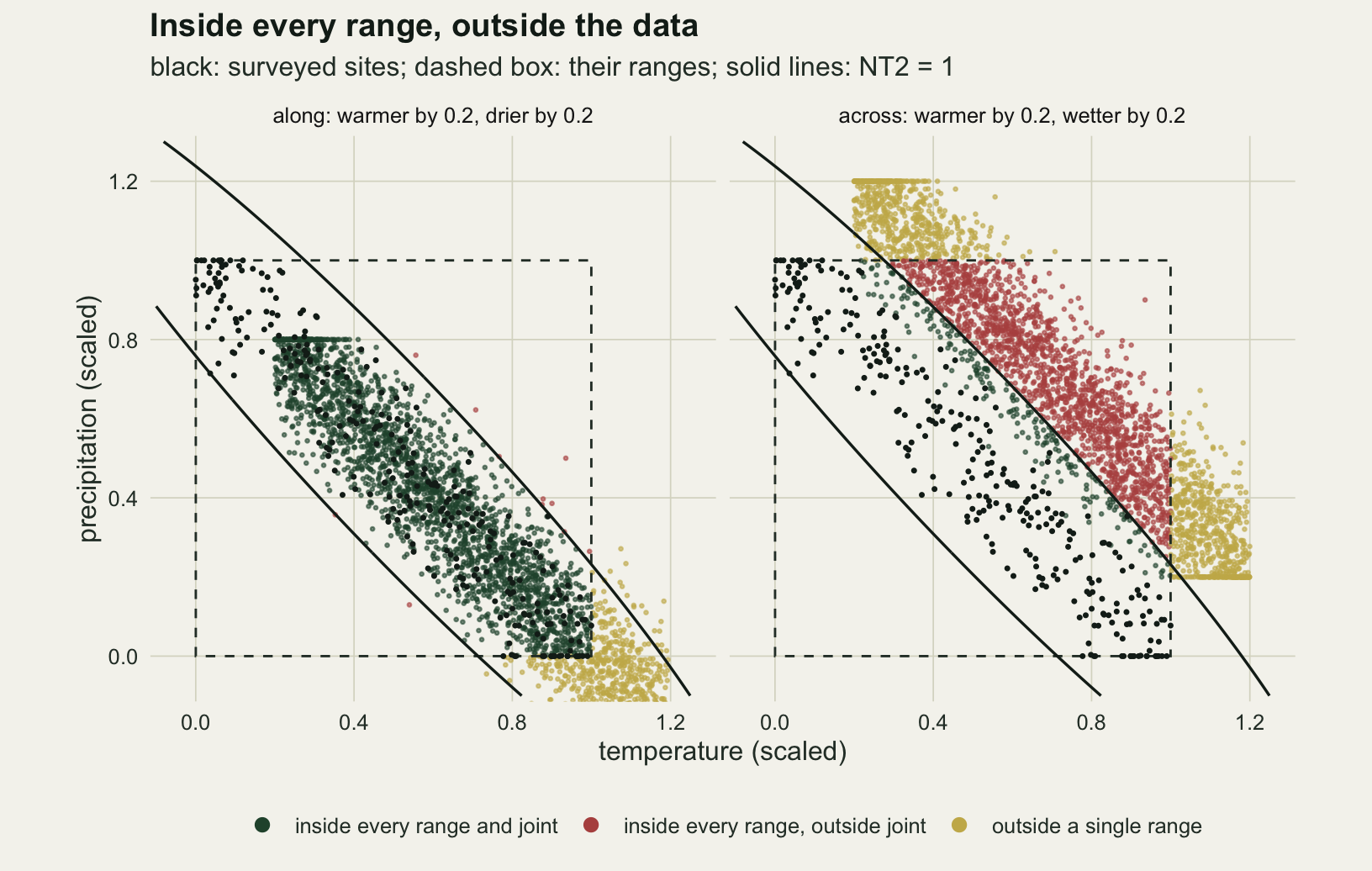
The figure shows why the two measures part company. The dashed box is what the MESS knows: the surveyed range of each covariate, which for a strip running corner to corner is nearly the whole square. The two solid lines are what NT2 knows: the long sides of an ellipse around the strip, too long to close inside the frame. The warmer and wetter future slides the strip towards the empty upper right of the box, and the part of it that crosses the upper line is inside the box and outside the joint region.
The rest of the NT2 story is the fragility of its threshold. NT2 against the training maximum is set by one site, the most extreme surveyed point, and that is why its across share varies from survey to survey as much as it does. Against the 99th percentile of the training distances instead, a threshold that ignores the three most extreme sites, NT2 flags 0.960 of the across cells (from 0.889 to 0.980), and the MESS-blind share becomes 0.557. The largest training distance was 1.06 to 1.46 times the 99th percentile in these surveys.
The full MESS of Elith and colleagues, with its percentile term, does not change the verdict either. Inside the range of a covariate that version scores a cell by twice the percentage of training values on its nearer side, which is positive for every value strictly inside the range; outside it uses the same edge distance as the stripped version. The two therefore agree on the sign, which is what the chunk above checks: the share of across cells on which they disagree is 0.000 in every survey. What the percentile term adds is a magnitude, and the blind cells are not marginal on it either: their median full MESS is 29.3, against 54.0 for the inside cells of the along future.
Two shifts of the same size
proj_stats <- function(fit, cells, f) {
  out <- c()
  for (nm in names(shifts)) {
    fut <- shift_cells(cells, shifts[[nm]])
    p_true_fut <- plogis(f(fut$temp, fut$prec))
    true_chg <- mean(p_true_fut) - mean(plogis(f(cells$temp, cells$prec)))
    pf <- predict(fit, fut, type = "link", se.fit = TRUE)
    pn <- predict(fit, cells, type = "link")
    err <- mean(plogis(pf$fit)) - mean(plogis(pn)) - true_chg
    covered <- p_true_fut >= plogis(pf$fit - 1.96 * pf$se.fit) &
               p_true_fut <= plogis(pf$fit + 1.96 * pf$se.fit)
    out <- c(out, setNames(c(err, mean(covered), true_chg),
                           paste(nm, c("err", "cov", "true"), sep = "_")))
  }
  out
}
glm_delta <- function(fit, cells, s) {
  b <- coef(fit); v_mat <- vcov(fit)
  x_now <- cbind(1, cells$temp, cells$prec)
  fut   <- shift_cells(cells, s)
  x_fut <- cbind(1, fut$temp, fut$prec)
  p_now <- plogis(drop(x_now %*% b)); p_fut <- plogis(drop(x_fut %*% b))
  grad <- colMeans(p_fut * (1 - p_fut) * x_fut) - colMeans(p_now * (1 - p_now) * x_now)
  sqrt(drop(t(grad) %*% v_mat %*% grad))
}
gam_delta <- function(fit, cells) {
  b <- coef(fit); v_mat <- vcov(fit)
  x_now <- predict(fit, cells, type = "lpmatrix")
  p_now <- plogis(drop(x_now %*% b))
  sapply(names(shifts), function(nm) {
    x_fut <- predict(fit, shift_cells(cells, shifts[[nm]]), type = "lpmatrix")
    p_fut <- plogis(drop(x_fut %*% b))
    grad <- colMeans(p_fut * (1 - p_fut) * x_fut) - colMeans(p_now * (1 - p_now) * x_now)
    sqrt(drop(t(grad) %*% v_mat %*% grad))
  })
}
glm_grad_ds <- function(fit, cells) {
  b <- coef(fit)
  b_ds <- c(b[[1]], (b[[2]] - b[[3]]) / 2, (b[[2]] + b[[3]]) / 2)
  x_ds <- function(z) cbind(1, z$temp - z$prec, z$temp + z$prec)
  p_now <- plogis(drop(x_ds(cells) %*% b_ds))
  grad <- function(s) {
    fut <- shift_cells(cells, s)
    p_fut <- plogis(drop(x_ds(fut) %*% b_ds))
    colMeans(p_fut * (1 - p_fut) * x_ds(fut)) - colMeans(p_now * (1 - p_now) * x_ds(cells))
  }
  c(g_along_def = abs(grad(shifts$along)[2]), g_across_sum = abs(grad(shifts$across)[3]),
    w_bar = mean(p_now * (1 - p_now)))
}

sim_rows <- list(); glm_rows <- list()
t_sim <- system.time({
  for (k in seq_len(n_draw)) {
    w <- draw_world(k)
    sites0  <- w$cells[w$idx, ]
    sites30 <- rbind(w$cells[w$idx[seq_len(n_site - n_off)], ], w$district)
    for (tn in names(truths)) {
      f <- truths[[tn]]
      arms <- if (tn %in% main_truths) c(0, 30) else if (k <= n_extra) 0 else numeric(0)
      for (arm in arms) {
        d_fit <- if (arm == 0) sites0 else sites30
        u_fit <- if (arm == 0) w$u_site else c(w$u_site[seq_len(n_site - n_off)], w$u_dist)
        d_fit$y <- as.integer(u_fit < plogis(f(d_fit$temp, d_fit$prec)))
        m_add <- gam(y ~ s(temp) + s(prec), family = binomial, data = d_fit, method = "REML")
        m_te  <- gam(y ~ te(temp, prec), family = binomial, data = d_fit, method = "REML")
        dm_add <- gam_delta(m_add, w$cells)
        sim_rows[[length(sim_rows) + 1]] <- data.frame(draw = k, truth = tn, arm = arm,
          model = "additive", t(proj_stats(m_add, w$cells, f)),
          dm_along = dm_add[["along"]], dm_across = dm_add[["across"]])
        sim_rows[[length(sim_rows) + 1]] <- data.frame(draw = k, truth = tn, arm = arm,
          model = "tensor", t(proj_stats(m_te, w$cells, f)), dm_along = NA, dm_across = NA)
        if (tn == "linear" && arm == 0) {
          m_glm <- glm(y ~ temp + prec, family = binomial, data = d_fit)
          glm_rows[[k]] <- data.frame(draw = k, t(proj_stats(m_glm, w$cells, f)),
            dm_along = glm_delta(m_glm, w$cells, shifts$along),
            dm_across = glm_delta(m_glm, w$cells, shifts$across),
            se_ratio = unname(sqrt(vcov(m_glm)[2, 2] + vcov(m_glm)[3, 3] + 2 * vcov(m_glm)[2, 3]) /
                              sqrt(vcov(m_glm)[2, 2] + vcov(m_glm)[3, 3] - 2 * vcov(m_glm)[2, 3])),
            t(glm_grad_ds(m_glm, w$cells)))
        }
      }
    }
  }
})
sim <- do.call(rbind, sim_rows)
glm_sim <- do.call(rbind, glm_rows)

cell_of <- function(tn, m, arm) sim[sim$truth == tn & sim$model == m & sim$arm == arm, ]
sd_err <- function(tn, m, arm, nm) sd(cell_of(tn, m, arm)[[paste0(nm, "_err")]])
rmse   <- function(x) sqrt(mean(x^2))
spread <- sapply(main_truths, function(tn)
  c(along = sd_err(tn, "additive", 0, "along"), across = sd_err(tn, "additive", 0, "across")))
ratio  <- spread["across", ] / spread["along", ]

set.seed(4460)
lin0 <- cell_of("linear", "additive", 0)
boot_ratio <- replicate(2000, {
  j <- sample.int(n_draw, replace = TRUE)
  sd(lin0$across_err[j]) / sd(lin0$along_err[j])
})
ratio_ci <- quantile(boot_ratio, c(0.025, 0.975))
along_rng <- sapply(main_truths, function(tn) range(cell_of(tn, "additive", 0)$along_err))
te_along_rng <- range(sim$along_err[sim$model == "tensor" & sim$truth %in% main_truths])
true_along <- sapply(main_truths, function(tn) median(cell_of(tn, "additive", 0)$along_true))
glm_sd <- c(along = sd(glm_sim$along_err), across = sd(glm_sim$across_err))
glm_dm <- c(along = median(glm_sim$dm_along), across = median(glm_sim$dm_across))
glm_grad <- c(along = median(glm_sim$g_along_def), across = median(glm_sim$g_across_sum),
              w04 = 0.4 * median(glm_sim$w_bar),
              ratio = median(glm_sim$g_across_sum / glm_sim$g_along_def))
gam_se <- function(tn, arm, nm) median(cell_of(tn, "additive", arm)[[paste0("dm_", nm)]])
k_worst <- which.max(abs(lin0$across_err))
worst_z <- abs(lin0$across_err[k_worst]) / lin0$dm_across[k_worst]
rmse_thr0 <- rmse(cell_of("threshold", "additive", 0)$across_err)
ratio_all <- sapply(names(truths), function(tn)
  sd_err(tn, "additive", 0, "across") / sd_err(tn, "additive", 0, "along"))
Each of the 20 surveys (seeds fixed before the runs) draws a new region, a new set of sites and new presences, and the same sites and random numbers serve all the species, so the species differ only in their truth. Two models are fitted to each survey by REML: the additive binomial GAM, a smooth of temperature plus a smooth of precipitation, and a tensor product smooth te() of the two. Each model then projects the change in mean occupancy over all 3000 cells under each future, and the error is that projection minus the true change. The spread of a projection is the standard deviation of this error over surveys.
For the additive model the along error has a standard deviation of 0.0062 on the threshold truth, 0.0044 on the unimodal truth and 0.0091 on the linear control. The true along changes being estimated are -0.178, -0.020 and -0.180, and the worst single survey missed by 0.012, 0.013 and 0.035 respectively. The across errors have standard deviations of 0.087, 0.087 and 0.096: ratios of 14.0, 19.6 and 10.5 to the along spread. The last one is the control, where the additive model is the right model. With 20 surveys the ratio is not sharply estimated: a bootstrap over surveys puts it between 5.7 and 24.4.
A projected change of zero for a warmer and wetter future is the right answer for every species here, and on the one truth where its form is correct the additive model misses it by up to 0.21 in mean occupancy. That is its worst survey of 20, and the miss is 2.5 times that survey’s own standard error. The fit does warn, if it is asked. The delta method applied to the GAM’s own coefficient covariance matrix gives a standard error of the across change with a median of 0.095 over surveys, the size of the spread itself, against 0.0067 along. A map drawn without that standard error hides the problem, and the agreement of fitted values that the collinearity post measures is a statement about the strip, not about how the strip is continued sideways. The warning covers the spread and not the bias: on the threshold truth the same standard error has a median of 0.097, while the root mean square error of the across change is 0.130.
The spread for a correctly specified model has a closed form, and it is worth writing down before reading anything into the ratio. Put the linear logistic model in the deficit and sum coordinates. Its slope along the sum is estimated from the scatter across the strip, and its standard error is larger than that of the slope along the deficit by the ratio of the spreads of the two coordinates among the sites, each weighted by the logistic variance p(1 - p). Unweighted and across the whole region, that ratio is 0.577 over 0.095, or 6.1; the weights concentrate the information where occupancy is near one half, which shortens the effective deficit range, and in the fitted models the ratio of the two standard errors has a median of 4.8. The delta method turns each slope’s standard error into a standard error of the projected change. For the logistic regression on temperature and precipitation, fitted to the same surveys of the linear species, it gives a median of 0.0067 along and 0.095 across, a ratio of 14.2, and the standard deviations over surveys were 0.0061 and 0.098.
The thin strip is only part of that ratio. The rest is how strongly each projected change responds to an error in its own slope. The across shift moves every cell 0.4 along the sum, so an error in the sum slope moves every cell’s projected change in logit by 0.4 times that error, and the change in mean occupancy responds with a gradient of about 0.4 times the mean of p(1 - p): 0.060 from the formula, 0.060 as the median of the computed gradients. The along change responds to an error in the deficit slope with a median gradient of only 0.020, because it is close to saturation. With a slope of 3 logit units per unit of deficit, occupancy already falls from near one to near zero across the region, so a steeper or shallower curve moves hardly more or less of the region from occupied to empty under the along shift. The sum slope is zero in truth, and near zero the across change grows in proportion to it, with nothing to saturate. The ratio of the two gradients has a median of 2.9, and its product with the median standard-error ratio of 4.8 is about 14, nearly all of the delta-method ratio. The logistic regression, which is exactly right for this species, has the across spread too, at almost the same size as the additive GAM, so the spread is not smoothing noise. It is fixed by the design, by how thin the strip is and how far the future leaves it. The GAM’s along spread, 0.0091, is larger than the logistic regression’s, which is the price of letting the smooths bend, and that is why its ratio is the smaller of the two.
The sign of the bias is the curvature
sym_split <- function(f, cells) {
  h <- function(deficit) f((deficit + 1) / 2, (1 - deficit) / 2)
  (h(2 * cells$temp - 1) + h(1 - 2 * cells$prec)) / 2
}
set.seed(4499)
ref_cells <- make_cells(n_cell)[1:1500, ]
ref_fut   <- shift_cells(ref_cells, shifts$across)
limit_tab <- t(sapply(names(truths), function(tn) {
  f <- truths[[tn]]
  formula_chg <- mean(plogis(sym_split(f, ref_fut))) - mean(plogis(sym_split(f, ref_cells)))
  ref_cells$p <- plogis(f(ref_cells$temp, ref_cells$prec))
  m_or <- suppressWarnings(gam(p ~ s(temp) + s(prec), family = quasibinomial,
                               data = ref_cells, method = "REML"))
  oracle_chg <- mean(predict(m_or, ref_fut, type = "response")) -
                mean(predict(m_or, ref_cells, type = "response"))
  a0 <- sim[sim$truth == tn & sim$arm == 0, ]
  c(formula = formula_chg, oracle = oracle_chg,
    add_med = median(a0$across_err[a0$model == "additive"]),
    add_lo  = min(a0$across_err[a0$model == "additive"]),
    add_hi  = max(a0$across_err[a0$model == "additive"]),
    add_mcse = 1.2533 * sd(a0$across_err[a0$model == "additive"]) /
               sqrt(sum(a0$model == "additive")),
    add_neg = mean(a0$across_err[a0$model == "additive"] < 0),
    te_med  = median(a0$across_err[a0$model == "tensor"]),
    te_lo   = min(a0$across_err[a0$model == "tensor"]),
    te_hi   = max(a0$across_err[a0$model == "tensor"]),
    te_pos  = sum(a0$across_err[a0$model == "tensor"] > 0),
    opp     = sum(sign(a0$across_err[a0$model == "tensor"]) !=
                  sign(a0$across_err[a0$model == "additive"])),
    n       = sum(a0$model == "tensor"))
}))
set.seed(4462)
n_ref_off <- 150
dist_limit <- replicate(5, {
  mix <- rbind(ref_cells[seq_len(nrow(ref_cells) - n_ref_off), c("temp", "prec")],
               data.frame(temp = runif(n_ref_off), prec = runif(n_ref_off)))
  mix$p <- plogis(truths$threshold(mix$temp, mix$prec))
  m_or <- suppressWarnings(gam(p ~ s(temp) + s(prec), family = quasibinomial,
                               data = mix, method = "REML"))
  mean(predict(m_or, ref_fut, type = "response")) -
    mean(predict(m_or, ref_cells, type = "response"))
})
lim_gap <- max(abs(limit_tab[, "formula"] - limit_tab[, "oracle"]))
med_gap <- max(abs(limit_tab[, "add_med"] - limit_tab[, "formula"]))
add_along_rng <- range(sim$along_err[sim$model == "additive" & sim$truth %in% main_truths])
The additive model is also biased across the strip, for every truth except the linear one, and the direction of the bias can be worked out before fitting anything. On the strip, a cell with deficit D sits at temperature (1 + D + e)/2 and precipitation (1 - D + e)/2, where e is its small scatter off the centre line. Write h(D) for the truth as a function of the deficit, on the logit scale. The split s(T) = h(2T - 1)/2, s(P) = h(1 - 2P)/2 reproduces the truth on the centre line and gives [h(D + e) + h(D - e)]/2 off it, an error of second order in e. Any other split adds a term proportional to e itself, which the scatter penalises, so with enough data the additive fit settles on this symmetric one. The across shift adds 0.4 to e, and the projection for a cell becomes
projected logit = [h(D + e + 0.4) + h(D - e - 0.4)] / 2, against a true logit of h(D).
That is the average of the truth at two points 0.4 either side of the true deficit, and its departure from the truth is a Jensen gap: negative where h is concave, positive where it is convex, zero where it is a straight line. A species with a threshold or an optimum along the water balance is concave on the logit scale, so the additive model projects a loss of occupancy that does not happen; a species favoured past a dryness threshold is convex, so it projects a gain; the linear species gets neither.
The chunk evaluates the formula on 1500 cells and checks it against an oracle, the additive GAM fitted to the true probabilities of the same cells with a quasibinomial likelihood, which is what the additive model would converge to with unlimited surveys. The formula gives projected changes of -0.075 for the threshold species, -0.017 for the weak threshold, +0.055 for the convex species, -0.171 for the unimodal species and +0.000 for the linear control; the oracle fit gives -0.078, -0.018, +0.055, -0.170 and -0.000. The largest difference is 0.002. The size of the gap is set by the curvature: the weak threshold, with the same kink and a slope of 3 instead of 10, has a limit a quarter the size or less.
d_seq <- seq(-1, 1, length.out = 401)
curve_df <- do.call(rbind, lapply(names(truths), function(tn) {
  f <- truths[[tn]]
  h <- function(deficit) f((deficit + 1) / 2, (1 - deficit) / 2)
  rbind(data.frame(truth = tn, deficit = d_seq, logit = h(d_seq),
                   curve = "truth, both futures"),
        data.frame(truth = tn, deficit = d_seq,
                   logit = (h(d_seq + 2 * a_shift) + h(d_seq - 2 * a_shift)) / 2,
                   curve = "additive limit, across future"))
}))
curve_df$truth <- factor(curve_df$truth, levels = names(truths))
curve_df$curve <- factor(curve_df$curve, levels = c("truth, both futures",
                                                    "additive limit, across future"))
ggplot(curve_df, aes(deficit, logit, colour = curve, linetype = curve)) +
  geom_line(linewidth = 0.9) +
  facet_wrap(~truth, ncol = 3, scales = "free_y", labeller = as_labeller(truth_lab)) +
  scale_colour_manual(values = c(te_ink, te_rust), name = NULL) +
  scale_linetype_manual(values = c("solid", "dashed"), name = NULL) +
  labs(x = "deficit, temperature minus precipitation", y = "logit of occupancy",
       title = "The additive projection averages the truth at two points",
       subtitle = "dashed: [h(D + 0.4) + h(D - 0.4)] / 2 at a cell on the centre line") +
  theme_datasheet() +
  theme(legend.position = "bottom")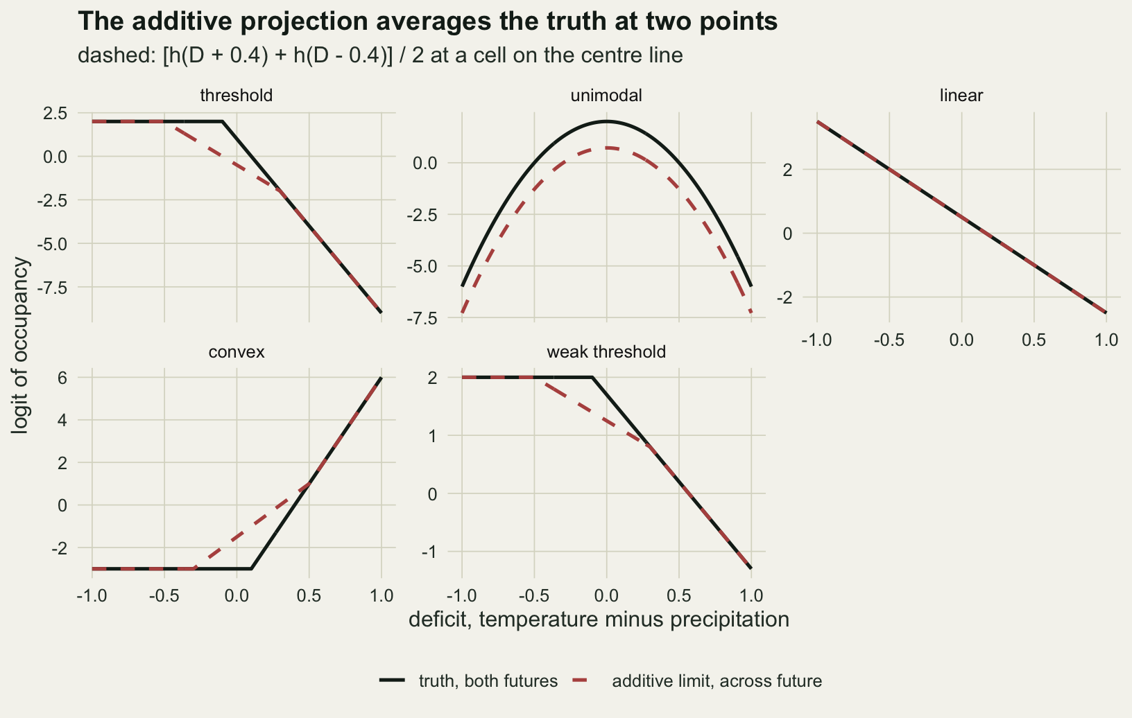
The formula is a limit. At 300 sites the additive model’s median across error is -0.088 for the threshold species, -0.036 for the weak threshold, +0.057 for the convex species, -0.150 for the unimodal species and -0.014 for the linear control, with ranges over surveys as wide as -0.267 to +0.087 for the unimodal species. The medians differ from the formula by at most 0.021, and that is as close as these runs can say: the Monte Carlo standard error of a median from 20 surveys (10 for the convex and weak threshold rows) is 0.024 to 0.041 here. The formula is checked against the oracle, not against these medians. The sign rule explains where the bias points; any one survey is dominated by the spread measured in the previous section.
err_df <- rbind(
  data.frame(sim[sim$arm == 0, c("draw", "truth", "model")], shift = "along",
             err = sim$along_err[sim$arm == 0]),
  data.frame(sim[sim$arm == 0, c("draw", "truth", "model")], shift = "across",
             err = sim$across_err[sim$arm == 0]))
err_df$row <- factor(paste(err_df$model, err_df$shift),
                     levels = rev(c("additive along", "additive across",
                                    "tensor along", "tensor across")))
err_df$truth <- factor(err_df$truth, levels = names(truths))
lim_df <- data.frame(truth = factor(rownames(limit_tab), levels = names(truths)),
                     formula = limit_tab[, "formula"],
                     row = factor("additive across", levels = levels(err_df$row)))
ggplot(err_df, aes(err, row)) +
  geom_vline(xintercept = 0, colour = te_body, linewidth = 0.3) +
  geom_jitter(aes(colour = shift), width = 0, height = 0.18, size = 1.3, alpha = 0.7) +
  geom_point(data = lim_df, aes(formula, row), shape = 124, size = 7, colour = te_rust) +
  facet_wrap(~truth, ncol = 3, labeller = as_labeller(truth_lab)) +
  scale_colour_manual(values = c(along = te_forest, across = te_gold),
                      breaks = c("along", "across"), name = NULL) +
  labs(x = "projected minus true change in mean occupancy", y = NULL,
       title = "Across the strip the projection scatters",
       subtitle = "one point per survey; 20 surveys for the first three truths, 10 for the last two") +
  theme_datasheet() +
  theme(legend.position = "bottom", panel.spacing = unit(1.2, "lines"))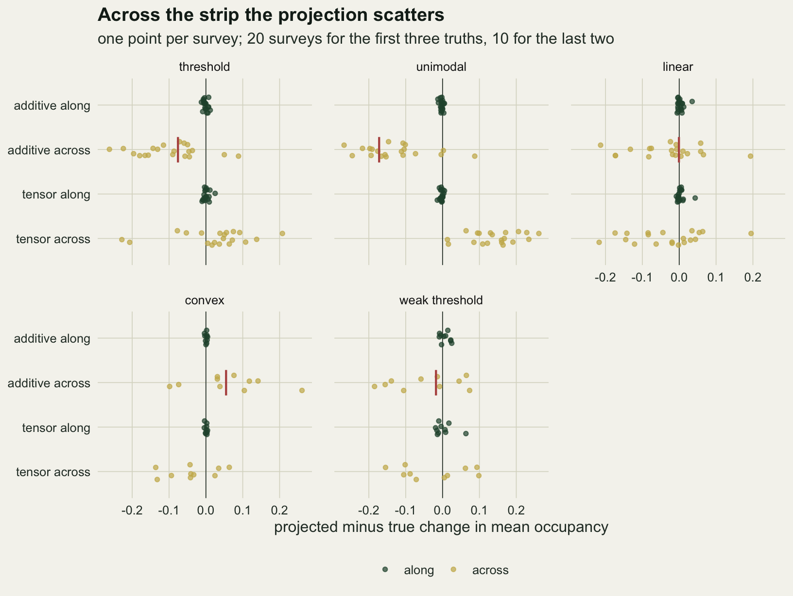
The tensor product smooth does not follow the rule, because it is not additive: it can represent a function of the deficit, and what it does off the strip depends on how its basis extrapolates. Its median across error is +0.043 for the threshold species, positive in 15 of 20 surveys, -0.019 for the linear species and +0.147 for the unimodal species, where it was positive in 20 of 20. The two models’ median errors have opposite signs for the threshold, convex and unimodal species, but survey by survey the signs differ in 18 of 20 surveys for the unimodal species, 13 of 20 for the threshold species and 5 of 10 for the convex one. A reliable reversal is a property of the unimodal truth, not a general rule: for the threshold species the tensor error straddles zero, from -0.228 to +0.208. Along the strip the tensor errors on the three main truths run from -0.014 to +0.054 over both arms of the design below, against -0.019 to +0.035 for the additive model.
A model given the deficit itself, a smooth of T - P and nothing else, would project a change of exactly zero across the strip for all five species, which is correct here. That is not a result about data. The truths were built as functions of the deficit, and a model in the deficit alone assumes that the sum has no effect at all, which is exactly the claim the survey cannot check. The failure measured here belongs to fitting temperature and precipitation as separate additive terms, the default in most climate envelope work, when the species responds to their combination.
cov_q <- function(tn, m, arm) q3(cell_of(tn, m, arm)$across_cov)
cov_thr  <- cov_q("threshold", "additive", 0)
cov_uni  <- cov_q("unimodal", "additive", 0)
cov_lin  <- cov_q("linear", "additive", 0)
cov_thr30 <- cov_q("threshold", "additive", 30)
cov_mean <- sapply(main_truths, function(tn) mean(cell_of(tn, "additive", 0)$across_cov))
lin_half <- sum(cell_of("linear", "additive", 0)$across_cov < 0.5)
The pointwise intervals are honest only for the linear control. The share of future cells whose true probability lies inside the model’s 95 per cent interval, with the cells of one survey as the denominator, has a median over surveys of 0.938 for the additive model on the threshold truth (from 0.310 to 1.000), 0.899 on the unimodal truth and 1.000 on the linear control. The medians flatter all three; the means are 0.869, 0.861 and 0.930. For the control the misses come in whole surveys: its worst survey covered 0.236 of the cells, and 2 of the 20 covered less than half, because the whole across region is one extrapolation that is right or wrong together, and an honest 95 per cent interval on one extrapolation should miss in about one survey in twenty. For the threshold and unimodal species the intervals are too narrow on average as well, because they carry the bias of the wrong form without allowing for it.
Thirty sites from somewhere else
rep_tab <- do.call(rbind, lapply(main_truths, function(tn) do.call(rbind, lapply(c("additive", "tensor"), function(m) {
  x0 <- cell_of(tn, m, 0); x30 <- cell_of(tn, m, 30)
  data.frame(truth = tn, model = m,
             rmse0 = rmse(x0$across_err), rmse30 = rmse(x30$across_err),
             bias0 = mean(x0$across_err), bias30 = mean(x30$across_err),
             sd0 = sd(x0$across_err), sd30 = sd(x30$across_err))
}))))
get_rep <- function(tn, m, col) rep_tab[rep_tab$truth == tn & rep_tab$model == m, col]
thr0  <- cell_of("threshold", "additive", 0)
thr30 <- cell_of("threshold", "additive", 30)
cut_thr <- 1 - rmse(thr30$across_err) / rmse(thr0$across_err)
set.seed(4461)
boot_cut <- replicate(2000, {
  j <- sample.int(n_draw, replace = TRUE)
  1 - rmse(thr30$across_err[j]) / rmse(thr0$across_err[j])
})
cut_ci <- quantile(boot_cut, c(0.025, 0.975))
blind30 <- q3(g30$across_blind)
bias_chg <- thr30$across_err - thr0$across_err
bias_chg_se <- sd(bias_chg) / sqrt(n_draw)
The obvious repair is data off the strip. Before any of the runs, the design of that data was fixed: 30 of the 300 sites are replaced by sites from a district where temperature and precipitation vary independently, each uniform on 0 to 1, as in a mountain block where aspect and elevation decouple the two. The district was not changed after the results were seen, and the bar for calling the repair useful was also set in advance: at least a quarter off the additive model’s across error on the threshold species, as root mean square error over surveys.
It clears that bar, narrowly. The additive model’s across RMSE on the threshold truth falls from 0.130 to 0.094, a cut of 28 per cent, with a bootstrap interval over surveys from -3 to 53 per cent, so the bar itself is inside the uncertainty. Its mean error moves from -0.099 to -0.075, a paired change of +0.024 with a standard error of 0.022 over the surveys, too noisy to show a shrinkage on its own. An oracle fit removes the survey noise. Fitted to the true probabilities, with no sampling noise, of 1350 strip cells and 150 district cells, the same one in ten, the additive model projects an across change of -0.101 to -0.049 over five draws of the district (median -0.068), against -0.078 with no district. The additive form is still wrong, so the bias stays in every draw; whether the district shrinks it or deepens it depends on where its few sites fall. The spread falls further. On the linear control the across standard deviation goes from 0.096 to 0.062, and on the threshold truth from 0.087 to 0.057. With the district in the training set the MESS-blind share falls to a median of 0.000. That is not because the strip has been filled in. The largest training distance is now a district site in 20 of 20 surveys, with a median of 5.40 against 2.06 for the largest among the strip sites, and against that strip maximum NT2 would still flag 0.871 of the across cells, a MESS-blind share of 0.479. The threshold moved far more than the coverage of the data did: this is the fragility of the maximum again.
The tensor model gains on the threshold species, from 0.103 to 0.072, and much less on the unimodal one, from 0.155 to 0.139, where its median error stays at +0.135.
There is a cost that the RMSE hides. With the district the across coverage of the additive model on the threshold truth falls from a median of 0.938 to 0.705, so its intervals narrowed by more than its error shrank. Its own standard error of the across change says the same: the median falls from 0.097 to 0.054, while the RMSE falls from 0.130 to 0.094. A wrong model with more data is more confidently wrong.
rep_long <- rbind(
  data.frame(rep_tab[, c("truth", "model")], sites = "0 decoupled sites", rmse = rep_tab$rmse0),
  data.frame(rep_tab[, c("truth", "model")], sites = "30 decoupled sites", rmse = rep_tab$rmse30))
rep_long$truth <- factor(rep_long$truth, levels = main_truths)
rep_long$lab <- factor(paste(rep_long$truth, rep_long$model, sep = ", "),
                       levels = rev(paste(rep(main_truths, each = 2),
                                          c("additive", "tensor"), sep = ", ")))
ggplot(rep_long, aes(rmse, lab)) +
  geom_line(aes(group = lab), colour = te_line, linewidth = 1.2) +
  geom_point(aes(colour = sites, shape = sites), size = 3) +
  scale_colour_manual(values = c(te_rust, te_forest), name = NULL) +
  scale_shape_manual(values = c(16, 17), name = NULL) +
  scale_x_continuous(limits = c(0, NA)) +
  labs(x = "RMSE of projected change, across future", y = NULL,
       title = "Decoupled sites shrink the across error, unevenly",
       subtitle = "20 surveys per point") +
  theme_datasheet() +
  theme(legend.position = "bottom")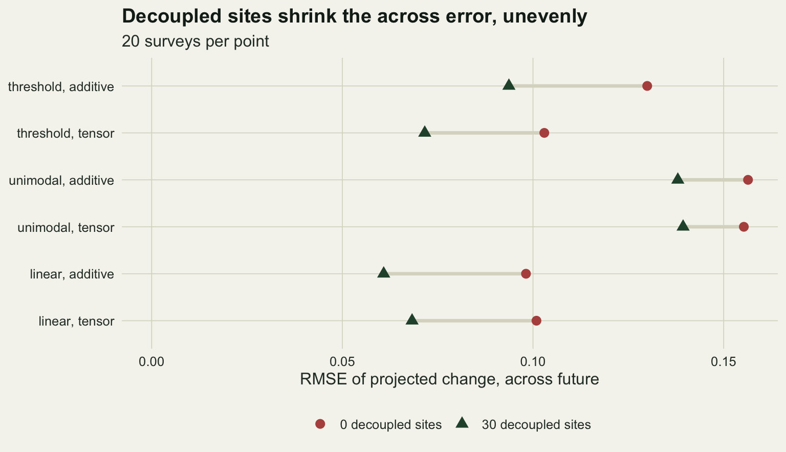
What to report
Report the correlation of the covariates in the survey and in the projection, not only the ranges. A single matrix of pairwise correlations for present and future, or a plot of the two most important covariates with the future cells on top, shows at once whether the future moves along the sampled cloud or off it; the one-covariate MESS map cannot. Here 0.502 of all the across future cells were inside on the MESS and outside everything sampled on NT2.
Map a joint-space novelty measure beside the MESS. NT2 from Mesgaran and colleagues is one Mahalanobis distance and one division. Say which threshold was used, the training maximum or a percentile, because on this design the flagged share moved from 0.893 to 0.960 between the two.
Treat a projected change in cells that the joint measure flags as extrapolation of the model’s form, not of the data. The correctly specified model’s spread across the strip was 10.5 times its spread along it here. The across spread follows from the design, so it can be estimated before any smooth is fitted: the delta method on a plain logistic regression gave 0.095, against 0.096 measured for the GAM. Report the delta-method standard error of the projected change beside the map, not only the map; it was honest for the correct form here, and for the threshold, unimodal and convex truths it was smaller than the actual error, because it cannot see a bias. Zurell and colleagues’ inflated response curves, which plot a model’s response across combinations of the other covariates that the data do not contain, are the matching check on the model side.
If the effect is plausibly carried by a combination of covariates, a water balance or a heat sum, fit that combination, and say that the projection then rests on the assumption that the other direction does not matter. If the projection must stand on separate terms, sample off the correlation. A small decoupled block cut the across error by 28 per cent here, and it narrowed the intervals by more than it shrank the error, so report coverage alongside.
Honest limits
Every truth depends on the deficit alone, so the across future has a true change of exactly zero. That makes the error easy to read and it is also the most favourable case for the sign rule: a truth with its own effect along the sum would add a real change to the Jensen gap and could mask it or add to it. The magnitude of the additive bias is tuned by the truths, as the weak threshold row shows; what carries over to other designs is the sign rule and the spread, not the numbers.
The strip is very thin. A correlation of -0.95 is at the strong end of what climate covariates show within a region, and the across spread of a correct model scales with the inverse of the weighted spread of the sum among the sites, so a weaker correlation, which widens the strip, gives a smaller one. A shift of 0.4 along the sum is also large against the scatter, and for the correct model the error in the projected logit grows in proportion to the shift.
The spread ratio rests on 20 surveys per cell, fixed in advance, and its bootstrap interval is wide. For the additive model the across spread is at least 7.1 times the along spread for all five truths, including the two run on 10 surveys; the ratio for any one truth is not known to better than the interval given.
NT2 against the training maximum depends on one site, and so does the MESS-blind share built on it. The percentile version is less fragile and flags more cells; neither has a threshold with a probabilistic meaning for a region like this one, and the shares should be read as geometry of this design, not as rates to expect elsewhere.
Two smoother families were fitted, both GAMs with default bases, plus the logistic regression used as a check. A boosted tree or MaxEnt with hinge features extrapolates differently off the strip, and the partial-dependence caveat in the tree ensemble check applies to their response curves. The decoupled district was one design, uniform over the whole square; a district placed where the future is expected to go might do more for the tensor model, and choosing it that way is a different, adaptive design that was not measured.
References
Williams JW, Jackson ST 2007 Frontiers in Ecology and the Environment 5(9):475-482 (10.1890/070037)
Dormann CF, Elith J, Bacher S, et al. 2013 Ecography 36(1):27-46 (10.1111/j.1600-0587.2012.07348.x)
Mesgaran MB, Cousens RD, Webber BL 2014 Diversity and Distributions 20(10):1147-1159 (10.1111/ddi.12209)
Elith J, Kearney M, Phillips S 2010 Methods in Ecology and Evolution 1(4):330-342 (10.1111/j.2041-210X.2010.00036.x)
Zurell D, Elith J, Schroeder B 2012 Diversity and Distributions 18(6):628-634 (10.1111/j.1472-4642.2012.00887.x)