library(ggplot2)
library(dplyr)Nest survival with logistic exposure in R
R
survival analysis
nest survival
ecology tutorial
Estimate daily nest survival in R with the logistic-exposure model, compare it against the Mayfield estimate, and let daily survival vary with nest age.
The apparent success of a set of nests, the fraction that fledge among those you found, is one of the most widely misreported numbers in field ecology. It overstates survival, because nests that fail early are less likely to be found in the first place, and because nests discovered late in the cycle have little exposure left in which to fail. Mayfield’s fix was to count survival per day of exposure rather than per nest, and the logistic-exposure model of Shaffer extends that idea into a generalised linear model, so daily survival can depend on nest age, date, habitat or weather. This post builds all three, the naive fraction, the Mayfield estimate and a logistic-exposure model, in base R, and shows the daily rate climbing with nest age in a way the constant-rate methods cannot see.
Nest monitoring intervals
Nest data arrive as visits. Between two visits a nest was exposed for some number of days and then was either still active or had failed. The unit of analysis is therefore the interval, carrying its length as an exposure and a binary outcome, survived or failed. The example is 220 nests of a bird with a 28-day cycle, found at varying ages and checked every three to five days, generated from a model in which daily survival improves as the nest ages.
The logistic-exposure model needs a link function that raises daily survival to the power of the interval length, so that a longer exposure has more chance to end in failure. Shaffer set this out in 2004; it is a one-off custom link passed to binomial.
logexp <- function(exposure = 1) {
  linkfun <- function(mu) qlogis(mu^(1 / exposure))
  linkinv <- function(eta) plogis(eta)^exposure
  mu.eta  <- function(eta) exposure * plogis(eta)^(exposure - 1) *
                           plogis(eta) * (1 - plogis(eta))
  valideta <- function(eta) TRUE
  structure(list(linkfun = linkfun, linkinv = linkinv, mu.eta = mu.eta,
                 valideta = valideta, name = "logexp"), class = "link-glm")
}set.seed(430)
period <- 28
dsr_true <- function(age) plogis(2.2 + 0.045 * age) # daily survival rises with age
n_nests <- 220
rows <- list(); fledged <- 0
for (i in seq_len(n_nests)) {
age <- sample(0:6, 1) # age when found
alive <- TRUE
while (age < period && alive) {
interval <- min(sample(3:5, 1), period - age)
survived <- 1L; fail_day <- NA
for (dd in seq_len(interval)) {
if (runif(1) > dsr_true(age + dd - 1)) { survived <- 0L; fail_day <- dd; break }
}
used <- if (survived == 1L) interval else fail_day
rows[[length(rows) + 1]] <- data.frame(nest = i, age_mid = age + used / 2,
exposure = used, survive = survived)
if (survived == 0L) alive <- FALSE else age <- age + interval
}
if (alive) fledged <- fledged + 1
}
d <- do.call(rbind, rows)
c(nests = n_nests, intervals = nrow(d), failures = sum(d$survive == 0),
exposure_days = sum(d$exposure)) nests intervals failures exposure_days
220 708 172 2449 The naive fraction and the Mayfield estimate
The naive apparent success is just the share of nests that fledged. The Mayfield estimate instead pools every failure against every exposure day to give a constant daily survival rate, then raises it to the length of the cycle.
naive_success <- fledged / n_nests
mayfield_dsr <- 1 - sum(d$survive == 0) / sum(d$exposure)
c(naive_apparent_success = round(naive_success, 3),
  mayfield_daily_survival = round(mayfield_dsr, 4),
  mayfield_period_survival = round(mayfield_dsr^period, 3))
naive_apparent_success mayfield_daily_survival mayfield_period_survival
0.2180 0.9298 0.1300 The naive fraction is about 0.22, while the Mayfield period survival is about 0.13. The naive figure runs high because nests found part way through the cycle only had to survive the days that remained, so counting them as full successes credits survival that was never observed. Pooling per exposure day removes that bias, and about 0.13 is the honest probability that a nest present on day zero reaches day 28, if daily survival were constant.
Letting daily survival vary with nest age
Constant daily survival is a strong claim. Eggs and small young are usually more vulnerable than nests about to fledge, so the daily rate should climb with age. Logistic exposure fits exactly that: a generalised linear model with the custom link, the interval outcome as response and nest age as a covariate.
m0 <- glm(survive ~ 1,       family = binomial(link = logexp(d$exposure)), data = d)
m1 <- glm(survive ~ age_mid, family = binomial(link = logexp(d$exposure)), data = d)
round(summary(m1)$coefficients, 4)
Estimate Std. Error z value Pr(>|z|)
(Intercept) 1.6357 0.1539 10.6258 0
age_mid 0.0829 0.0138 6.0016 0c(AIC_constant = round(AIC(m0), 1), AIC_age = round(AIC(m1), 1),
delta_AIC = round(AIC(m0) - AIC(m1), 1))AIC_constant AIC_age delta_AIC
965.5 923.5 42.0 The age coefficient is about 0.083 on the logit scale with a standard error near 0.014, so daily survival rises reliably with age, and the age model beats the constant one by about 42 AIC units. Translating the fit back to daily survival shows the size of the change across the cycle.
b <- coef(m1)
ages <- c(2, 14, 26)
data.frame(age = ages,
           fitted_DSR = round(plogis(b[1] + b[2] * ages), 3),
           true_DSR = round(dsr_true(ages), 3))
age fitted_DSR true_DSR
1 2 0.858 0.908
2 14 0.942 0.944
3 26 0.978 0.967Daily survival climbs from roughly 0.86 for a two-day-old nest to about 0.98 for one near fledging, tracking the values that generated the data at the middle and upper ages. A constant rate averages across that gradient and so overstates the danger to old nests while understating it for young ones. The plotted curve makes the trend and its uncertainty explicit against the flat Mayfield rate.
nd <- data.frame(age_mid = seq(0, period, by = 0.5))
pr <- predict(m1, nd, type = "link", se.fit = TRUE)
nd$dsr <- plogis(pr$fit)
nd$lo <- plogis(pr$fit - 1.96 * pr$se.fit)
nd$hi <- plogis(pr$fit + 1.96 * pr$se.fit)

ggplot(nd, aes(age_mid, dsr)) +
  geom_ribbon(aes(ymin = lo, ymax = hi), fill = te_forest, alpha = 0.16) +
  geom_hline(yintercept = mayfield_dsr, colour = te_gold, linetype = "42", linewidth = 0.8) +
  geom_line(colour = te_forest, linewidth = 1.0) +
  annotate("text", x = 1, y = mayfield_dsr - 0.012, label = "constant Mayfield rate",
           colour = "#8a7a30", hjust = 0, size = 3.1) +
  annotate("text", x = 20, y = 0.955, label = "logistic-exposure fit",
           colour = te_forest, hjust = 0, size = 3.1) +
  labs(title = "Daily nest survival rises with age",
       subtitle = "The exposure model recovers a gradient the constant rate cannot show",
       x = "Nest age (days)", y = "Daily survival rate") +
  theme_te()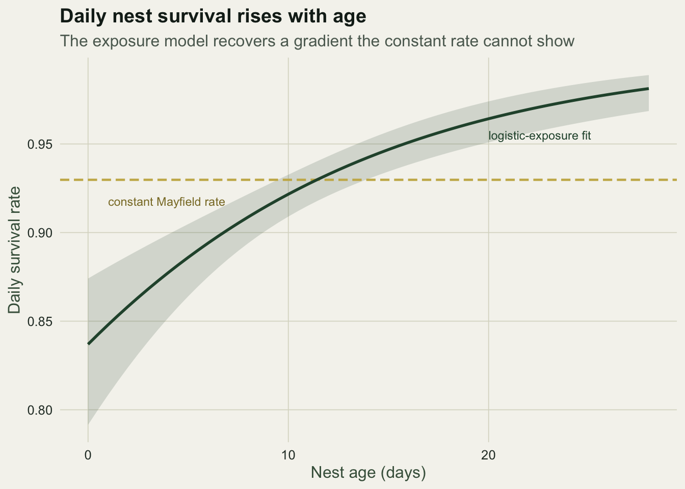
Survival across the whole cycle
Multiplying the age-specific daily rates across the 28 days gives the probability a nest survives the cycle, and comparing it with the constant-rate version shows where the two diverge: they part most over the vulnerable early days.
day <- 0:period
surv_age  <- c(1, cumprod(plogis(b[1] + b[2] * (0:(period - 1)))))
surv_const <- mayfield_dsr^day
pdf <- bind_rows(
  data.frame(day = day, S = surv_age,  model = "Age-varying (logistic exposure)"),
  data.frame(day = day, S = surv_const, model = "Constant (Mayfield)"))

ggplot(pdf, aes(day, S, colour = model)) +
  geom_line(linewidth = 0.95) +
  scale_colour_manual(values = c("Age-varying (logistic exposure)" = te_forest,
                                 "Constant (Mayfield)" = te_gold)) +
  annotate("text", x = 28, y = surv_age[period + 1] + 0.05, label = "age-varying",
           colour = te_forest, hjust = 1, size = 3.1) +
  annotate("text", x = 20, y = 0.24, label = "constant", colour = "#8a7a30", hjust = 0, size = 3.1) +
  coord_cartesian(ylim = c(0, 1)) +
  labs(title = "Survival across the nesting cycle",
       subtitle = "Age-specific daily rates compound differently from a single pooled rate",
       x = "Day of cycle", y = "Cumulative survival") +
  theme_te()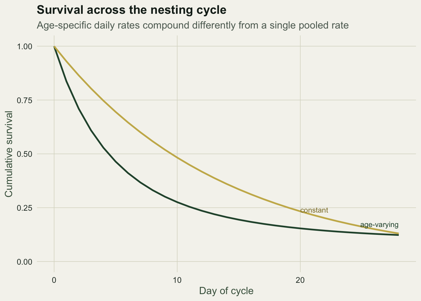
Both paths end near a period survival of about 0.12, far below the naive 0.22, but they get there differently: the constant curve falls too fast at the start and too slowly at the end, because it cannot know that the earliest days carry most of the risk. For questions that turn on timing, when to concentrate predator control, or how habitat shifts the daily rate, the exposure model is the one that answers them.
Where to go next
Logistic exposure is an ordinary generalised linear model with a purpose-built link, so everything from binomial regression carries over: additional covariates, interactions and the same care with separation and overdispersion. It shares the exposure logic of an offset for rates and densities, where a count is modelled per unit of effort rather than per record, and it sits alongside the other survival tools here, the Kaplan-Meier curve and the Cox model for known fates, and the Cormack-Jolly-Seber model when survival must be inferred from recaptures.
References
Mayfield HF 1975. The Wilson Bulletin 87(4):456-466 (10.2307/4160682).
Johnson DH 1979. The Auk 96(4):651-661 (10.1093/auk/96.4.651).
Shaffer TL 2004. The Auk 121(2):526-540 (10.1093/auk/121.2.526).
Dinsmore SJ, White GC, Knopf FL 2002. Ecology 83(12):3476-3488 (10.1890/0012-9658(2002)083[3476:ATFMAN]2.0.CO;2).