library(ggplot2)
library(patchwork)

te_paper  <- "#f5f4ee"
te_ink    <- "#16241d"
te_body   <- "#2c3a31"
te_forest <- "#275139"
te_rust   <- "#b5534e"
te_gold   <- "#c9b458"
te_line   <- "#dad9ca"

theme_datasheet <- function() {
  theme_minimal(base_size = 12) +
    theme(plot.background  = element_rect(fill = te_paper, colour = NA),
          panel.background = element_rect(fill = te_paper, colour = NA),
          panel.grid.major = element_line(colour = te_line, linewidth = 0.3),
          panel.grid.minor = element_blank(),
          text             = element_text(colour = te_body),
          plot.title       = element_text(colour = te_ink, face = "bold"),
          plot.subtitle    = element_text(colour = te_body),
          axis.text        = element_text(colour = te_body),
          strip.text       = element_text(colour = te_ink))
}Model discrepancy in simulator calibration
R
simulation models
Gaussian processes
calibration
model misspecification
ecology tutorial
Calibrating a linear intake simulator against a saturating truth in R: a GP discrepancy stays honest only while its amplitude is set from outside the data.
A shorebird foraging model is built around one assumption about intake: a bird walking a mudflat takes cockles at a rate proportional to their density, so intake is an attack rate times density. The simulator then runs days, tides and a whole wintering population on that line. The attack rate is not known, so it is calibrated against feeding trials in which captive birds are offered cockles at a range of densities and the intake is timed. The trouble is that a real bird has to open each shell. Handling time bends the true intake curve below the line, gently at low density and more at high density, and no value of the attack rate makes the simulator’s straight line go through the trial data.
That is the calibration problem Kennedy and O’Hagan wrote down in 2001: reality equals the simulator at the right parameter value plus a model discrepancy, a function of the input that the simulator does not contain, given a Gaussian process prior. Emulating a slow simulation model builds the other half of their framework, the Gaussian process that stands in for a simulator too slow to run often, and says in its closing limits that it stops well short of calibrating anything against field data. This post starts where that one stops. The simulator here is fast and needs no emulator; the question is what the discrepancy term does to the calibrated parameter.
Two other posts on this site sit next to the question. Light response curves: the curvature you drop shows that fitting a curve of the wrong shape gives a bias that is a projection of the truth onto the wrong family, fixed by the design and not a feature of the noise. That is the plain least-squares calibration here, and it is given one line below rather than a section. Starting values and identifiability in nls ends on parameters that the data cannot separate however the fit is started. A discrepancy flexible enough to absorb any error in the simulator produces exactly that situation for the attack rate, and the likelihood has no way to tell the two apart.
None of the results below are new. Brynjarsdottir and O’Hagan (2014) used this very pair, a simulator theta x against a reality theta x / (1 + x / a), to show that a discrepancy with a vague prior leaves the physical parameter unlearned and that realistic learning about it needs prior information about the discrepancy itself, and they imposed the same zero value and zero slope at the origin that is used below (together with monotonicity). Tuo and Wu (2015) showed that the Kennedy and O’Hagan parameter is not in general the value that makes the simulator closest to reality, and Plumlee (2017) proposed a discrepancy prior orthogonal to the simulator’s gradient so that the parameter has a definite meaning. The constants here differ from theirs: an attack rate of 1.2, a saturation constant of 10, trial densities from 0.1 to 4 and an observation standard deviation of 0.05 that is treated as known. What the post measures is how each of those arguments looks in coverage, standard errors and sample size, and one thing that software defaults decide without asking: whether the size of the discrepancy is fixed in advance or estimated from the trial data it is meant to correct.
A linear simulator and a saturating truth
The true intake is the Holling type II form theta x / (1 + x / 10) with theta = 1.2, which is the disc equation of Functional responses in R written with the attack rate in front. The simulator is theta x. Trials are equally spaced over densities 0.1 to 4 and the intake is measured with independent normal error of standard deviation 0.05. The discrepancy is a squared-exponential Gaussian process, as in Gaussian process regression from scratch, and for any fixed amplitude and length-scale the calibrated attack rate is a generalised least-squares estimate with the discrepancy covariance plus the observation variance as its covariance matrix.
The constrained version, as Brynjarsdottir and O’Hagan did, conditions that process on two facts a behavioural ecologist knows before any trial is run: at zero density both the true intake and the simulator are zero, so the discrepancy is zero there, and at vanishing density a bird is not yet limited by handling, so the discrepancy has zero slope at zero as well. A squared-exponential process and its derivative are jointly Gaussian, and conditioning on the value and the derivative at zero gives a closed-form covariance, which is the k_con function below.
theta_true <- 1.2
sat_k      <- 10
sd_obs     <- 0.05
x_lo       <- 0.1
x_hi       <- 4
n_set      <- c(10, 30, 90, 270)
amp_fix    <- 1
len_fix    <- 1.5
z_95       <- qnorm(0.975)

bound_log       <- 6
x_in            <- 2.05
x_out           <- 6
n_rep_ml        <- c(`10` = 200, `30` = 200, `90` = 200, `270` = 60)
n_rep_bayes     <- 100
amp_prior_sd    <- 1
len_prior_med   <- 1.5
len_prior_sdlog <- 0.75

eta_fun <- function(x, a0 = 0) a0 + theta_true * x / (1 + x / sat_k)
x_design <- function(n) seq(x_lo, x_hi, length.out = n)

k_se <- function(a, b, amp, len) {
  amp^2 * exp(-outer(a, b, "-")^2 / (2 * len^2))
}
k_con <- function(a, b, amp, len) {
  ga <- exp(-a^2 / (2 * len^2))
  gb <- exp(-b^2 / (2 * len^2))
  k_se(a, b, amp, len) - amp^2 * (outer(ga, gb) + outer(ga * a, gb * b) / len^2)
}
k_none <- function(a, b, amp, len) matrix(0, length(a), length(b))
k_pick <- function(kind) switch(kind, none = k_none, gp = k_se, con = k_con)

cov_obs <- function(kind, x, amp, len) {
  k_pick(kind)(x, x, amp, len) + diag(sd_obs^2, length(x))
}set.seed(4102)
n_demo <- 30
x_demo <- x_design(n_demo)
y_demo <- eta_fun(x_demo) + rnorm(n_demo, 0, sd_obs)
ls_demo <- sum(x_demo * y_demo) / sum(x_demo^2)
gap_4 <- theta_true * x_hi - eta_fun(x_hi)
gap_pct <- 100 * gap_4 / eta_fun(x_hi)
proj_theta <- integrate(function(x) x * eta_fun(x), x_lo, x_hi)$value /
integrate(function(x) x^2, x_lo, x_hi)$valueAt the highest trial density the truth sits 1.37 below the true-rate line, 40 per cent of the true intake there. On one simulated set of 30 trials the least-squares attack rate is 0.922. The no-discrepancy calibration is the case the light response post already covers: its target is the projection of the truth onto straight lines through the origin, which over the trial range is 0.9266, and its interval shrinks around the projection at the design points, which approaches that value as trials are added, so it never covers 1.2 at any n in the table below.
x_line <- seq(0, 6, length.out = 200)
curve_df <- rbind(
  data.frame(x = x_line, y = eta_fun(x_line), what = "truth, saturating"),
  data.frame(x = x_line, y = ls_demo * x_line, what = "simulator, least squares"),
  data.frame(x = x_line, y = theta_true * x_line, what = "simulator, true attack rate"))
ggplot(curve_df, aes(x, y, colour = what, linetype = what)) +
  annotate("rect", xmin = x_hi, xmax = 6, ymin = -Inf, ymax = Inf,
           fill = te_line, alpha = 0.45) +
  geom_line(linewidth = 0.9) +
  geom_point(data = data.frame(x = x_demo, y = y_demo), aes(x, y),
             inherit.aes = FALSE, colour = te_ink, size = 1.6) +
  scale_colour_manual(values = c(te_gold, te_rust, te_forest), name = NULL) +
  scale_linetype_manual(values = c("solid", "dashed", "solid"), name = NULL) +
  labs(x = "prey density", y = "intake rate",
       title = "A straight line against a gentle bend",
       subtitle = "shaded: beyond the trial densities, where the simulator will be used") +
  theme_datasheet() +
  theme(legend.position = "bottom")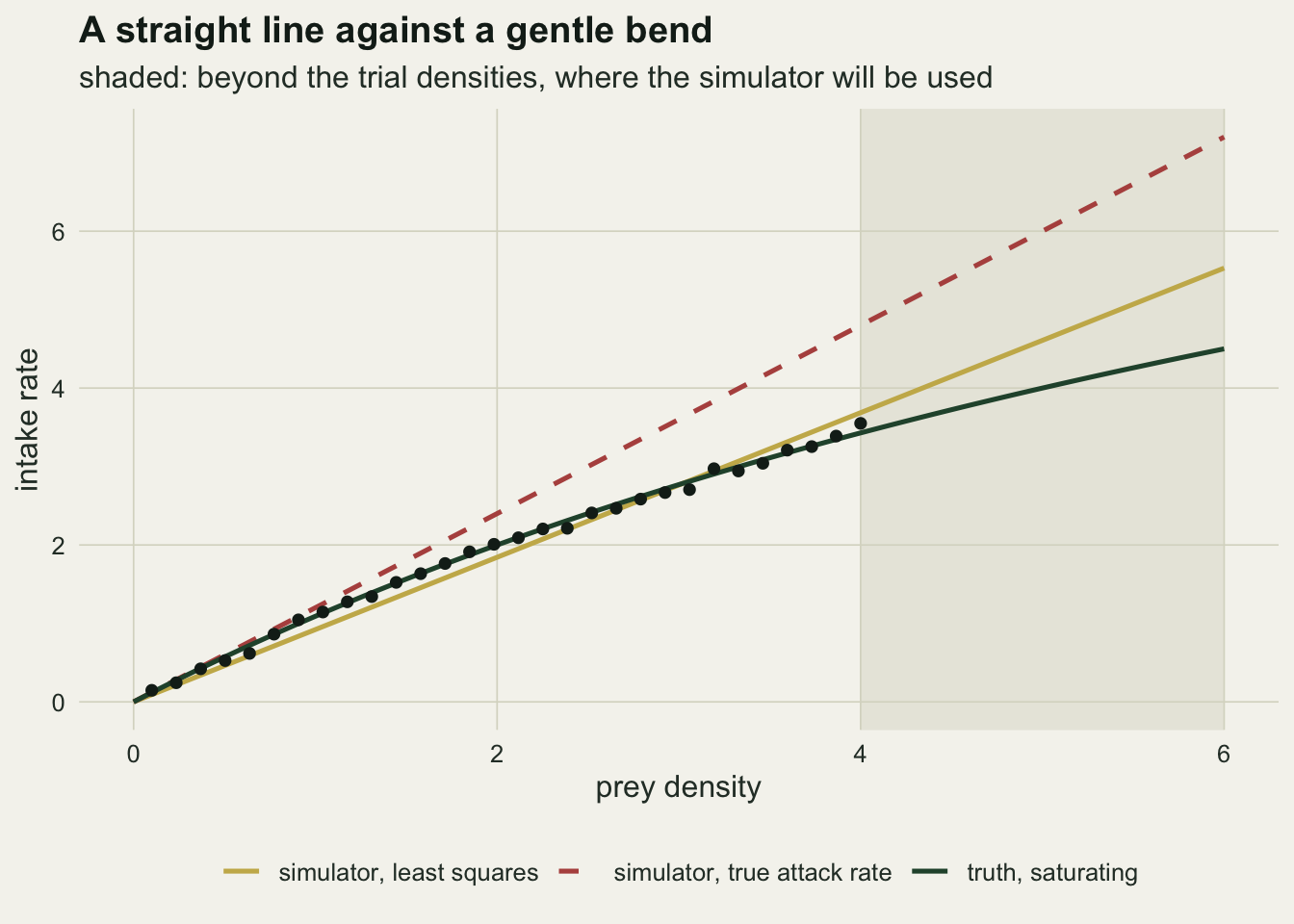
The straight line fitted by least squares passes through the trial data closely enough that a residual plot from thirty points would not raise much alarm. Its slope is well below the true attack rate, and beyond the trial range, where a foraging model is run at densities the trials never offered, the fitted line and the truth separate.
With the hyperparameters fixed, the table is arithmetic
Fix the discrepancy amplitude at 1 and the length-scale at 1.5. An amplitude of 1 is generous next to a true intake that rises to 3.43 over the trials, and those are the values used before any data were simulated. With both fixed, every arm is a linear estimator of the data: a weight vector w times y. Its mean is w times the true curve, its sampling standard deviation is 0.05 times the length of w, and the standard error it reports is the GLS value. Coverage then follows from two normal probabilities, and none of the table below comes from a simulation.
linear_arm <- function(kind, n, amp = amp_fix, len = len_fix, a0 = 0,
                       target = theta_true) {
  x  <- x_design(n)
  kx <- solve(cov_obs(kind, x, amp, len), x)
  v  <- 1 / sum(x * kx)
  w  <- v * kx
  m  <- sum(w * eta_fun(x, a0))
  sd_w <- sd_obs * sqrt(sum(w^2))
  se <- sqrt(v)
  data.frame(n = n, arm = kind, mean = m, se = se, sd_true = sd_w,
             cover = pnorm((target - m + z_95 * se) / sd_w) -
                     pnorm((target - m - z_95 * se) / sd_w),
             sum_w = sum(w))
}
cf_tab <- do.call(rbind, lapply(n_set, function(n)
  do.call(rbind, lapply(c("none", "gp", "con"), linear_arm, n = n))))
cf_get <- function(arm, n, col) cf_tab[cf_tab$arm == arm & cf_tab$n == n, col]

n_check <- 400
set.seed(733)
x_chk  <- x_design(30)
ch_chk <- lapply(c(gp = "gp", con = "con"),
                 function(kind) chol(cov_obs(kind, x_chk, amp_fix, len_fix)))
gls_chol <- function(ch, x, y) {
  xs <- backsolve(ch, x, transpose = TRUE)
  ys <- backsolve(ch, y, transpose = TRUE)
  v  <- 1 / sum(xs^2)
  c(est = v * sum(xs * ys), se = sqrt(v))
}
chk <- replicate(n_check, {
  y <- eta_fun(x_chk) + rnorm(30, 0, sd_obs)
  sapply(ch_chk, function(ch) {
    g <- gls_chol(ch, x_chk, y)
    c(g, hit = abs(g[["est"]] - theta_true) < z_95 * g[["se"]])
  })
})
chk_cover <- apply(chk["hit", , ], 1, mean)
chk_mean  <- apply(chk["est", , ], 1, mean)
chk_mcse  <- sqrt(chk_cover * (1 - chk_cover) / n_check)
knitr::kable(cf_tab[, c("n", "arm", "mean", "se", "cover")], digits = 3,
row.names = FALSE)| n | arm | mean | se | cover |
|---|---|---|---|---|
| 10 | none | 0.916 | 0.007 | 0.000 |
| 10 | gp | 0.856 | 0.223 | 0.950 |
| 10 | con | 1.081 | 0.126 | 0.933 |
| 30 | none | 0.923 | 0.004 | 0.000 |
| 30 | gp | 0.857 | 0.219 | 0.931 |
| 30 | con | 1.126 | 0.092 | 0.934 |
| 90 | none | 0.925 | 0.002 | 0.000 |
| 90 | gp | 0.856 | 0.213 | 0.930 |
| 90 | con | 1.151 | 0.066 | 0.940 |
| 270 | none | 0.926 | 0.001 | 0.000 |
| 270 | gp | 0.853 | 0.208 | 0.927 |
| 270 | con | 1.170 | 0.047 | 0.952 |
A check that the closed form is right: 400 simulated datasets at n = 30 give coverage 0.938 for the unconstrained discrepancy and 0.935 for the constrained one (Monte Carlo standard errors 0.012 and 0.012), against 0.931 and 0.934 from the formula, with mean estimates 0.855 and 1.125 against 0.857 and 1.126.
The unconstrained discrepancy buys nominal coverage, 0.950 at 10 trials and 0.927 at 270, and it buys it by not learning. Its mean estimate is 0.856 at 10 trials and 0.853 at 270, further from 1.2 than plain least squares, and its standard error goes from 0.223 to 0.208 while the number of trials rises twenty-sevenfold. That plateau is what Brynjarsdottir and O’Hagan describe: a discrepancy that can take any smooth shape can also take the shape of a change in the attack rate, so more trials inform the sum and not its parts. The interval is honest only because it is as wide as the prior on the discrepancy allows.
The constrained discrepancy behaves differently. The estimate moves from 1.081 at 10 trials to 1.170 at 270, the standard error falls from 0.126 to 0.047, and the coverage stays between 0.933 and 0.952. Near zero density a discrepancy with zero value and zero slope cannot imitate a change in slope, so the low-density trials pin the attack rate. The estimate is still below 1.2 at 270 trials; the interval covers because the bias shrinks alongside the standard error, not because it has gone.
arm_lab <- c(none = "no discrepancy", gp = "GP discrepancy",
             con = "GP, zero value and slope at zero density")
cf_plot <- cf_tab
cf_plot$arm_name <- factor(arm_lab[cf_plot$arm], levels = arm_lab)
ggplot(cf_plot, aes(factor(n), mean, colour = arm_name)) +
  geom_hline(yintercept = theta_true, linetype = "dashed", colour = te_ink) +
  geom_errorbar(aes(ymin = mean - z_95 * se, ymax = mean + z_95 * se),
                width = 0.25, linewidth = 0.8,
                position = position_dodge(width = 0.6)) +
  geom_point(size = 2.4, position = position_dodge(width = 0.6)) +
  scale_colour_manual(values = c(te_rust, te_gold, te_forest), name = NULL) +
  labs(x = "feeding trials (n)", y = "attack rate",
       title = "Fixed hyperparameters: honest, but only one arm learns",
       subtitle = "dashed: the true attack rate") +
  guides(colour = guide_legend(nrow = 2)) +
  theme_datasheet() +
  theme(legend.position = "bottom")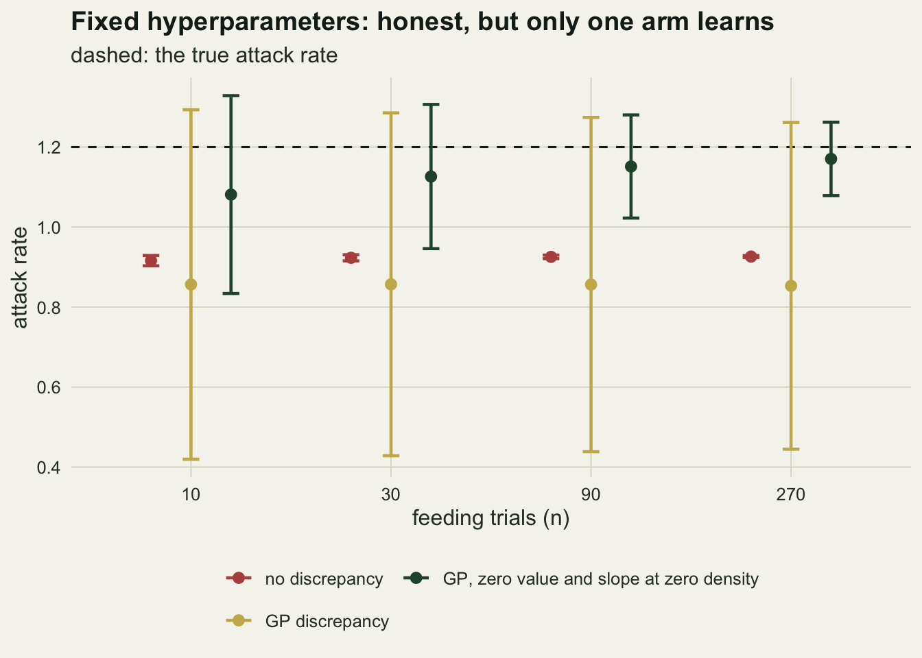
Learning the discrepancy from the same data
Nobody running a calibration package types an amplitude of 1. The default is to estimate the discrepancy hyperparameters, and the cheapest way, used here, is maximum likelihood (type II): maximise the likelihood of the trial data over the log amplitude and log length-scale, with the attack rate profiled out by GLS at each step. Kennedy and O’Hagan themselves plugged in estimated hyperparameters rather than integrating over them. The optimiser is Nelder-Mead run from four starting points (amplitude and length-scale 0.5 and 1, 5 and 5, 0.05 and 0.3, 2 and 10), keeping the fit with the highest likelihood, with both log parameters kept inside plus or minus 6. The run uses 200 datasets at each of 10, 30 and 90 trials and 60 at 270, to keep the knit short; each dataset is also calibrated with the fixed hyperparameters so the two can be compared on the same draws.
starts_log <- list(c(log(0.5), log(1)), c(log(5), log(5)),
                   c(log(0.05), log(0.3)), c(log(2), log(10)))

fit_hyper <- function(kind, x, y) {
  sq_dist <- outer(x, x, "-")^2
  x_prod  <- outer(x, x)
  nll <- function(p) {
    if (any(abs(p) > bound_log)) return(1e10)
    amp <- exp(p[1])
    len <- exp(p[2])
    kmat <- exp(-sq_dist / (2 * len^2))
    if (kind == "con") {
      g <- exp(-x^2 / (2 * len^2))
      kmat <- kmat - outer(g, g) * (1 + x_prod / len^2)
    }
    ch <- tryCatch(chol(amp^2 * kmat + diag(sd_obs^2, length(x))),
                   error = function(e) NULL)
    if (is.null(ch)) return(1e10)
    xs <- backsolve(ch, x, transpose = TRUE)
    ys <- backsolve(ch, y, transpose = TRUE)
    r  <- ys - xs * sum(xs * ys) / sum(xs^2)
    0.5 * sum(r^2) + sum(log(diag(ch)))
  }
  fits <- lapply(starts_log, function(s)
    optim(s, nll, control = list(maxit = 200, reltol = 1e-6)))
  vals <- vapply(fits, function(o) o$value, numeric(1))
  opt  <- fits[[which.min(vals)]]
  c(amp = exp(opt$par[1]), len = exp(opt$par[2]),
    at_bound = any(abs(opt$par) > bound_log - 0.05),
    first_worse = vals[1] - min(vals) > 0.01)
}

predict_arm <- function(kind, x, y, amp, len, a0 = 0) {
  kfun <- k_pick(kind)
  ch <- chol(cov_obs(kind, x, amp, len))
  solve_k <- function(b) backsolve(ch, backsolve(ch, b, transpose = TRUE))
  kx  <- solve_k(x)
  v   <- 1 / sum(x * kx)
  est <- v * sum(kx * y)
  x_new <- c(x_in, x_out)
  ks  <- kfun(x_new, x, amp, len)
  p_mean <- drop(x_new * est + ks %*% solve_k(y - x * est))
  p_var  <- diag(kfun(x_new, x_new, amp, len)) -
    rowSums(ks * t(solve_k(t(ks)))) + drop(x_new - ks %*% kx)^2 * v
  p_sd <- sqrt(pmax(p_var, 0))
  hit  <- abs(p_mean - eta_fun(x_new, a0)) < z_95 * p_sd
  c(est = est, se = sqrt(v), hit_in = hit[1], hit_out = hit[2],
    psd_in = p_sd[1], psd_out = p_sd[2])
}

set.seed(9150)
ml_rows <- list()
for (n in n_set) {
  x  <- x_design(n)
  mu <- eta_fun(x)
  for (i in seq_len(n_rep_ml[[as.character(n)]])) {
    y <- mu + rnorm(n, 0, sd_obs)
    for (kind in c("gp", "con")) {
      hp <- fit_hyper(kind, x, y)
      ml_rows[[length(ml_rows) + 1]] <- data.frame(
        n = n, arm = kind, fit = "estimated", t(hp),
        t(predict_arm(kind, x, y, hp[["amp"]], hp[["len"]])))
      ml_rows[[length(ml_rows) + 1]] <- data.frame(
        n = n, arm = kind, fit = "fixed", amp = amp_fix, len = len_fix,
        at_bound = 0, first_worse = 0,
        t(predict_arm(kind, x, y, amp_fix, len_fix)))
    }
  }
}
ml_all <- do.call(rbind, ml_rows)
ml_all$hit <- abs(ml_all$est - theta_true) < z_95 * ml_all$se

ml_sum <- do.call(rbind, lapply(split(ml_all, list(ml_all$n, ml_all$arm, ml_all$fit)),
  function(d) data.frame(n = d$n[1], arm = d$arm[1], fit = d$fit[1],
                         reps = nrow(d), mean = mean(d$est), se = mean(d$se),
                         cover = mean(d$hit),
                         mcse = sqrt(mean(d$hit) * (1 - mean(d$hit)) / nrow(d)),
                         amp = median(d$amp), len = median(d$len),
                         at_bound = mean(d$at_bound),
                         first_worse = mean(d$first_worse),
                         cover_in = mean(d$hit_in), cover_out = mean(d$hit_out),
                         psd_in = mean(d$psd_in), psd_out = mean(d$psd_out))))
ml_sum <- ml_sum[order(ml_sum$fit, ml_sum$arm, ml_sum$n), ]
ml_get <- function(arm, fit, n, col) {
  ml_sum[ml_sum$arm == arm & ml_sum$fit == fit & ml_sum$n == n, col]
}
knitr::kable(ml_sum[ml_sum$fit == "estimated",
                    c("n", "arm", "reps", "mean", "se", "cover", "amp", "len", "at_bound",
                      "first_worse")],
digits = 3, row.names = FALSE)| n | arm | reps | mean | se | cover | amp | len | at_bound | first_worse |
|---|---|---|---|---|---|---|---|---|---|
| 10 | con | 200 | 1.148 | 0.030 | 0.545 | 403.330 | 61.997 | 0.845 | 0.375 |
| 30 | con | 200 | 1.164 | 0.022 | 0.415 | 403.155 | 62.150 | 0.670 | 0.225 |
| 90 | con | 200 | 1.177 | 0.017 | 0.645 | 8.012 | 8.999 | 0.315 | 0.075 |
| 270 | con | 60 | 1.182 | 0.012 | 0.767 | 8.990 | 9.174 | 0.083 | 0.033 |
| 10 | gp | 200 | 0.872 | 0.044 | 0.000 | 0.178 | 1.484 | 0.000 | 0.075 |
| 30 | gp | 200 | 0.867 | 0.046 | 0.000 | 0.188 | 1.667 | 0.000 | 0.080 |
| 90 | gp | 200 | 0.860 | 0.052 | 0.000 | 0.224 | 1.941 | 0.000 | 0.080 |
| 270 | gp | 60 | 0.853 | 0.059 | 0.000 | 0.287 | 2.254 | 0.000 | 0.083 |
The unconstrained discrepancy collapses. Its median fitted amplitude is 0.178 at 10 trials and 0.287 at 270, less than three tenths of the value fixed above, and with a small discrepancy the estimate is again forced to carry the misfit. The mean estimate stays at 0.872 to 0.853, but the reported standard error is now 0.044 at 10 trials and 0.059 at 270, between 0.20 and 0.28 of its fixed-amplitude value. The interval covers the true attack rate in 0 of 200 datasets at 10 trials, 0 of 200 at 90 and 0 of 60 at 270. The same trial data, calibrated with a fixed amplitude, covered in a fraction 0.950 of the datasets at 90 trials. The only difference is where the size of the discrepancy came from.
The reported standard error is 2.9 times the scatter of the estimates: across the datasets at 90 trials the standard deviation of the estimated-hyperparameter estimate is 0.018, against a mean reported standard error of 0.052. The interval fails on location, not on width: both numbers are small next to a bias of 0.340.
The constrained discrepancy with estimated hyperparameters is in between. Its coverage is 0.545, 0.415, 0.645 and 0.767 at 10, 30, 90 and 270 trials, with mean estimates from 1.148 to 1.182. Its hyperparameters behave differently from the unconstrained ones: the fitted amplitude and length-scale run off together along a ridge towards large values, where the constrained process looks like a curvature term with a variance of its own, and at 10 and 30 trials 85 and 67 per cent of fits ended at the bound on the log parameters. The likelihood is nearly flat along that ridge, so the bound itself changes little; a wider bound on the log parameters, tried outside the post, gave the same coverage within Monte Carlo error. The starting point is not harmless. The first start on its own stopped at a worse optimum (log-likelihood lower by more than 0.01) in 38 and 22 per cent of datasets at 10 and 30 trials, against 7 per cent for the unconstrained discrepancy at 10 trials, which is why every fit keeps the best of four starts.
est_long <- rbind(
  data.frame(ml_sum[, c("n", "arm", "fit")], metric = "coverage of the true rate",
             value = ml_sum$cover, lo = pmax(ml_sum$cover - 2 * ml_sum$mcse, 0),
             hi = pmin(ml_sum$cover + 2 * ml_sum$mcse, 1)),
  data.frame(ml_sum[, c("n", "arm", "fit")], metric = "mean standard error",
             value = ml_sum$se, lo = NA, hi = NA))
est_long$arm_name <- factor(ifelse(est_long$arm == "gp", "GP discrepancy",
                                   "GP, zero value and slope at zero"),
                            levels = c("GP discrepancy", "GP, zero value and slope at zero"))
est_long$fit <- factor(est_long$fit, levels = c("fixed", "estimated"),
                       labels = c("amplitude 1, length 1.5 fixed", "estimated by maximum likelihood"))
ref_df <- data.frame(metric = "coverage of the true rate", value = 0.95)
ggplot(est_long, aes(n, value, colour = fit)) +
  geom_hline(data = ref_df, aes(yintercept = value), linetype = "dashed",
             colour = te_ink) +
  geom_line(linewidth = 0.8) +
  geom_errorbar(aes(ymin = lo, ymax = hi), width = 0.08, linewidth = 0.5,
                na.rm = TRUE) +
  geom_point(size = 2.3) +
  facet_grid(metric ~ arm_name, scales = "free_y", switch = "y") +
  scale_x_log10(breaks = n_set) +
  expand_limits(y = 0) +
  scale_colour_manual(values = c(te_forest, te_rust), name = NULL) +
  labs(x = "feeding trials (n)", y = NULL,
       title = "Learning the discrepancy from the same data",
       subtitle = "bars: two Monte Carlo standard errors; dashed: 0.95") +
  theme_datasheet() +
  theme(legend.position = "bottom", strip.placement = "outside")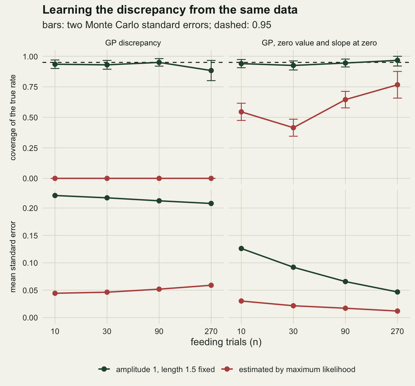
The lower panels show the mechanism in standard errors. The two fixed-amplitude arms differ in slope: flat for the unconstrained discrepancy, falling for the constrained one. Estimating the hyperparameters moves both curves down, and for the unconstrained discrepancy it moves it far below the size of the bias.
Prediction of intake inside the trial range mostly survives this. At a density of 2.05 the 95 per cent prediction interval for the true intake covers it in between 0.850 and 0.970 of datasets across all four arms and all sample sizes, because the discrepancy absorbs much of what the attack rate gets wrong; the lowest value is the unconstrained discrepancy with estimated hyperparameters at 270 trials, from 60 datasets. Outside the range it does not. At a density of 6 the unconstrained discrepancy with estimated hyperparameters covers the true intake in 0.190 to 0.267 of datasets, and even the constrained discrepancy with fixed hyperparameters falls from 0.885 at 10 trials to 0.383 at 270. The only arm that covers there, in at least 0.995 of datasets, is the unconstrained discrepancy with its amplitude fixed at 1, and it does so with a mean prediction standard deviation of 0.96 at 90 trials against a true intake of 4.50.
Would a weak prior have saved it?
An objection to the section above is fair: maximum likelihood is not what a Bayesian calibration does. A full calibration puts a prior on the hyperparameters and integrates over them. That can be done exactly on a grid for this problem. A flat prior on the attack rate integrates out analytically, leaving the restricted likelihood of each hyperparameter pair; the prior used is half-normal with scale 1 on the amplitude and lognormal with median 1.5 and log-scale standard deviation 0.75 on the length-scale, over an 18 by 18 grid with amplitude from 0.02 to 5 and length-scale from 0.2 to 12, and the posterior for the attack rate is the resulting mixture of normals. The grid bounds are part of the prior.
la_grid <- seq(log(0.02), log(5), length.out = 18)
ll_grid <- seq(log(0.2), log(12), length.out = 18)
hyper_grid <- expand.grid(la = la_grid, ll = ll_grid)
log_prior <- -exp(2 * hyper_grid$la) / (2 * amp_prior_sd^2) + hyper_grid$la +
  dnorm(hyper_grid$ll, log(len_prior_med), len_prior_sdlog, log = TRUE)

bayes_rows <- list()
set.seed(6628)
for (n in c(30, 90)) {
  x  <- x_design(n)
  mu <- eta_fun(x)
  chols <- lapply(c(gp = "gp", con = "con"), function(kind)
    lapply(seq_len(nrow(hyper_grid)), function(j)
      chol(cov_obs(kind, x, exp(hyper_grid$la[j]), exp(hyper_grid$ll[j])))))
  for (i in seq_len(n_rep_bayes)) {
    y <- mu + rnorm(n, 0, sd_obs)
    for (kind in c("gp", "con")) {
      grid_fit <- t(vapply(chols[[kind]], function(ch) {
        xs <- backsolve(ch, x, transpose = TRUE)
        ys <- backsolve(ch, y, transpose = TRUE)
        v  <- 1 / sum(xs^2)
        est <- v * sum(xs * ys)
        r  <- ys - xs * est
        c(ll = -0.5 * sum(r^2) - sum(log(diag(ch))) + 0.5 * log(v),
          est = est, se = sqrt(v))
      }, numeric(3)))
      lw <- grid_fit[, "ll"] + log_prior
      wt <- exp(lw - max(lw))
      wt <- wt / sum(wt)
      post_cdf <- function(th) sum(wt * pnorm(th, grid_fit[, "est"], grid_fit[, "se"]))
      lo <- uniroot(function(th) post_cdf(th) - 0.025, c(-5, 5))$root
      hi <- uniroot(function(th) post_cdf(th) - 0.975, c(-5, 5))$root
      bayes_rows[[length(bayes_rows) + 1]] <- data.frame(
        n = n, arm = kind, mean = sum(wt * grid_fit[, "est"]), lo = lo, hi = hi,
        amp_post = sum(wt * exp(hyper_grid$la)))
    }
  }
}
bayes_all <- do.call(rbind, bayes_rows)
bayes_all$hit <- bayes_all$lo < theta_true & bayes_all$hi > theta_true
bayes_sum <- do.call(rbind, lapply(split(bayes_all, list(bayes_all$n, bayes_all$arm)),
  function(d) data.frame(n = d$n[1], arm = d$arm[1], mean = mean(d$mean),
                         width = mean(d$hi - d$lo), cover = mean(d$hit),
                         mcse = sqrt(mean(d$hit) * (1 - mean(d$hit)) / nrow(d)),
                         amp_post = mean(d$amp_post))))
by_get <- function(arm, n, col) bayes_sum[bayes_sum$arm == arm & bayes_sum$n == n, col]
knitr::kable(bayes_sum, digits = 3, row.names = FALSE)| n | arm | mean | width | cover | mcse | amp_post |
|---|---|---|---|---|---|---|
| 30 | con | 1.137 | 0.258 | 0.84 | 0.037 | 1.269 |
| 90 | con | 1.160 | 0.159 | 0.88 | 0.032 | 1.408 |
| 30 | gp | 0.860 | 0.545 | 0.10 | 0.030 | 0.556 |
| 90 | gp | 0.854 | 0.551 | 0.03 | 0.017 | 0.612 |
The weak prior does not save the unconstrained discrepancy. Its equal-tailed 95 per cent posterior interval is 0.545 wide on average at 30 trials, wider than the maximum likelihood interval, yet it contains 1.2 in 0.10 of the 100 datasets at 30 trials and 0.03 at 90 (Monte Carlo standard errors 0.030 and 0.017). The posterior mean amplitude is 0.56 at 30 trials: the data still pull the amplitude well below the prior scale, and the posterior mean attack rate stays at 0.860.
With the constraint, the same prior does most of the repair. Maximum likelihood gave this arm coverage of 0.415 at 30 trials; integrating over the grid gives 0.84 at 30 trials and 0.88 at 90 (standard errors 0.037 and 0.032), still below 0.95, and the interval narrows from 0.258 to 0.159. So in this example integrating over the hyperparameters matters for the constrained discrepancy, and it is the constraint, not the prior on the amplitude, that decides whether the attack rate can be learned at all.
When the constraint is only nearly true
The constraint used above is exactly true of the chosen truth, which flatters it. Suppose instead that the trials record a small intake even at zero density, from a timing convention or from birds taking a few cockles missed in the tray count, so the truth is 0.05 + theta x / (1 + x / 10). The intercept is one observation standard deviation. The constrained discrepancy is still told that the discrepancy is zero at zero density, which is now false by 0.05.
A different kind of prior information is a discrepancy orthogonal to the simulator’s gradient, as Plumlee proposed. Here the gradient of the simulator with respect to the attack rate is x, so the constraint is that the integral of x times the discrepancy over the trial range is zero, imposed on the same squared-exponential process through a 400-point quadrature. Both cases are linear estimators with fixed hyperparameters, so they are closed form again.
a0_small <- 0.05
q_n  <- 400
q_x  <- x_lo + (seq_len(q_n) - 0.5) * (x_hi - x_lo) / q_n
q_wx <- rep((x_hi - x_lo) / q_n, q_n) * q_x
k_orth <- function(a, b, amp, len) {
  ka <- k_se(a, q_x, amp, len) %*% q_wx
  kb <- k_se(b, q_x, amp, len) %*% q_wx
  k_se(a, b, amp, len) - ka %*% t(kb) / drop(t(q_wx) %*% k_se(q_x, q_x, amp, len) %*% q_wx)
}
k_pick <- function(kind) switch(kind, none = k_none, gp = k_se, con = k_con,
                                orth = k_orth)
near_tab <- do.call(rbind, lapply(n_set, function(n) rbind(
  cbind(linear_arm("con", n, a0 = a0_small), case = "constrained, small intercept"),
  cbind(linear_arm("gp", n, a0 = a0_small), case = "unconstrained, small intercept"),
  cbind(linear_arm("orth", n), case = "orthogonal, true rate"),
  cbind(linear_arm("orth", n, target = proj_theta), case = "orthogonal, projection"))))
nr_get <- function(case, n, col) near_tab[near_tab$case == case & near_tab$n == n, col]
knitr::kable(near_tab[, c("n", "case", "mean", "se", "cover", "sum_w")], digits = 3,
row.names = FALSE)| n | case | mean | se | cover | sum_w |
|---|---|---|---|---|---|
| 10 | constrained, small intercept | 1.187 | 0.126 | 0.996 | 2.125 |
| 10 | unconstrained, small intercept | 0.867 | 0.223 | 0.967 | 0.218 |
| 10 | orthogonal, true rate | 0.926 | 0.007 | 0.000 | 0.374 |
| 10 | orthogonal, projection | 0.926 | 0.007 | 0.951 | 0.374 |
| 30 | constrained, small intercept | 1.262 | 0.092 | 0.952 | 2.721 |
| 30 | unconstrained, small intercept | 0.867 | 0.219 | 0.952 | 0.211 |
| 30 | orthogonal, true rate | 0.926 | 0.004 | 0.000 | 0.375 |
| 30 | orthogonal, projection | 0.926 | 0.004 | 0.950 | 0.375 |
| 90 | constrained, small intercept | 1.313 | 0.066 | 0.624 | 3.225 |
| 90 | unconstrained, small intercept | 0.866 | 0.213 | 0.953 | 0.204 |
| 90 | orthogonal, true rate | 0.927 | 0.002 | 0.000 | 0.375 |
| 90 | orthogonal, projection | 0.927 | 0.002 | 0.950 | 0.375 |
| 270 | constrained, small intercept | 1.359 | 0.047 | 0.036 | 3.768 |
| 270 | unconstrained, small intercept | 0.863 | 0.208 | 0.954 | 0.200 |
| 270 | orthogonal, true rate | 0.927 | 0.001 | 0.000 | 0.375 |
| 270 | orthogonal, projection | 0.927 | 0.001 | 0.950 | 0.375 |
The intercept breaks the constrained calibration and the damage grows with the number of trials. The estimate is 1.187 at 10 trials and 1.359 at 270, above the true 1.2, and coverage falls from 0.996 to 0.624 at 90 trials and 0.036 at 270. The weights explain it. Constrained GLS weights sum to 2.13 at 10 trials and 3.77 at 270, so an intercept of 0.05 adds that multiple of 0.05 to the estimate, while the standard error shrinks. The unconstrained discrepancy shrugs the intercept off (coverage 0.954 at 270 trials) for the same reason it never learned anything.
The orthogonal discrepancy gives a definite answer, and it is not 1.2. Its estimate is 0.9266 at 270 trials with a standard error of 0.0013, the same as plain least squares, and its interval covers the least-squares projection 0.9266 in 0.950 of datasets and the true attack rate in 0.000. That is the point of the construction: it makes the calibrated parameter the best-fitting simulator value in the sense of the L2 projection, the target Tuo and Wu adopt for an imperfect simulator. For a foraging model the question is then which quantity is wanted. The rate a bird attacks at before handling limits it is 1.2; the slope that makes a straight-line model match intake over densities 0.1 to 4 is 0.927. No discrepancy prior turns one into the other; the choice is made before the data are seen.
near_plot <- rbind(
  cbind(cf_tab[cf_tab$arm == "con", c("n", "mean", "se")],
        case = "constraint exactly true"),
  near_tab[near_tab$case == "constrained, small intercept", c("n", "mean", "se", "case")],
  near_tab[near_tab$case == "orthogonal, projection", c("n", "mean", "se", "case")])
near_plot$case <- factor(near_plot$case,
  levels = c("constraint exactly true", "constrained, small intercept", "orthogonal, projection"),
  labels = c("constrained, truth passes through zero", "constrained, truth has intercept 0.05",
             "orthogonal discrepancy"))
ggplot(near_plot, aes(factor(n), mean, colour = case)) +
  geom_hline(yintercept = theta_true, linetype = "dashed", colour = te_ink) +
  geom_hline(yintercept = proj_theta, linetype = "dotted", colour = te_ink) +
  geom_errorbar(aes(ymin = mean - z_95 * se, ymax = mean + z_95 * se),
                width = 0.25, linewidth = 0.8,
                position = position_dodge(width = 0.6)) +
  geom_point(size = 2.4, position = position_dodge(width = 0.6)) +
  scale_colour_manual(values = c(te_forest, te_rust, te_gold), name = NULL) +
  labs(x = "feeding trials (n)", y = "attack rate",
       title = "The constraint is information, and it can be wrong",
       subtitle = "dashed: true rate; dotted: least-squares projection of the truth") +
  guides(colour = guide_legend(nrow = 2)) +
  theme_datasheet() +
  theme(legend.position = "bottom")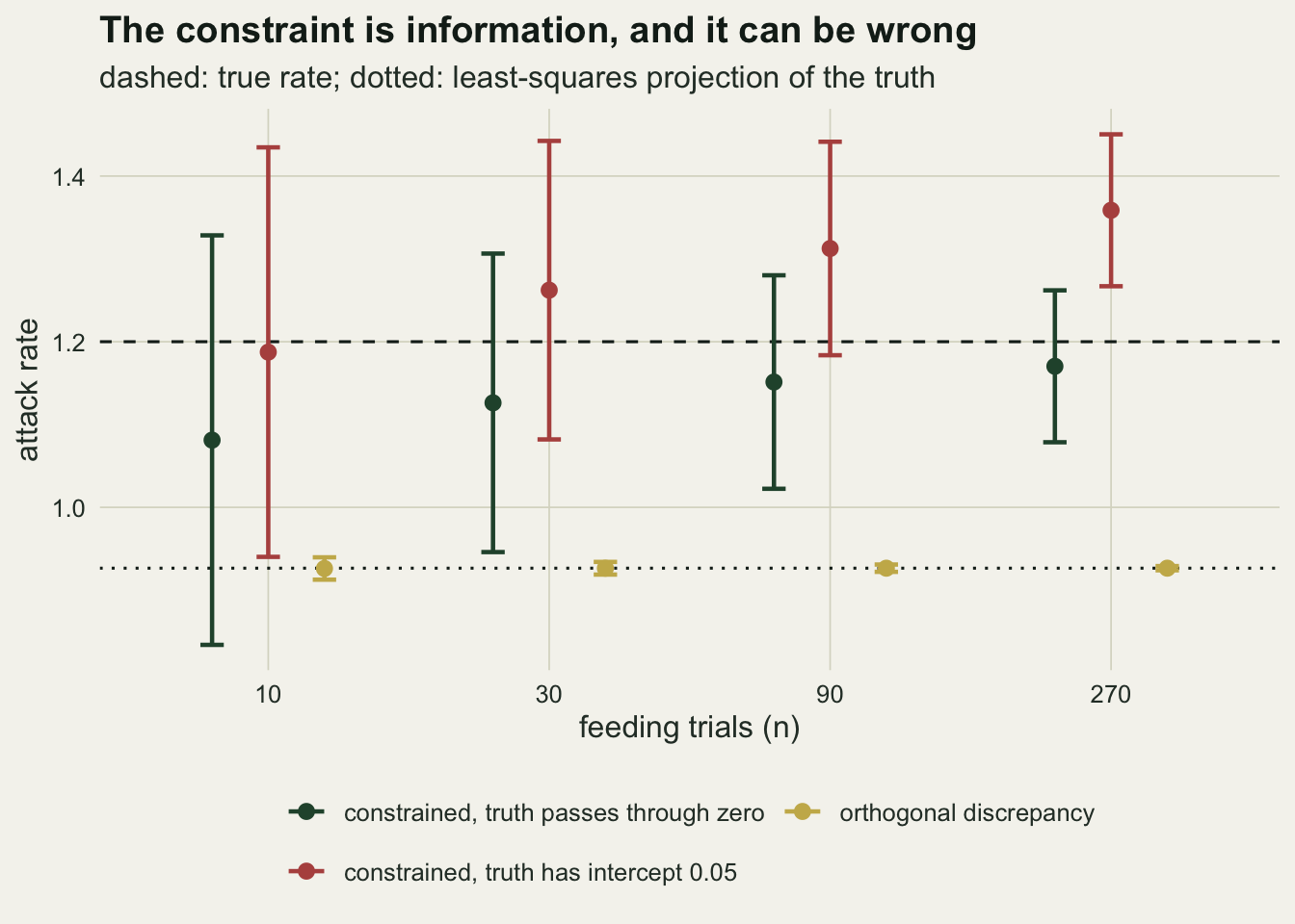
What to report
Say where the discrepancy hyperparameters came from. A calibrated parameter with a Gaussian process discrepancy is a different quantity when the amplitude is fixed from prior knowledge than when it is estimated from the same data, and in this example the difference was coverage near 0.95 against coverage of zero on identical datasets. A methods sentence of the form “a GP discrepancy was included” is not enough to read the interval.
Report the standard error of the parameter at two sample sizes, or its behaviour with added data, when the data allow it. A standard error that does not fall as trials are added means the discrepancy is absorbing the parameter, and the parameter is being reported from its prior.
State the prior information about the discrepancy as a claim about the system and defend it on ecological grounds: here, that intake and the simulator agree at zero density and that handling does not limit intake at vanishing density. Then check what happens if the claim is slightly wrong. In the intercept case above a violation of one observation standard deviation was enough to take coverage from nominal to 0.036 at 270 trials.
Say which parameter is meant. If the target is the physical attack rate, the calibration needs information about the discrepancy from outside the data. If the target is the best-fitting simulator value, plain least squares or an orthogonal discrepancy estimates it, and the report should call it that and not the attack rate.
Keep prediction inside the calibration range apart from extrapolation. Inside the range the prediction intervals covered in 0.850 to 0.970 of datasets across the arms; at a density of 6 only the arm with the widest intervals covered at every sample size, and a foraging model is usually run exactly where the trials were not.
Honest limits
One simulator, one truth and one input dimension. The simulator is linear in its single parameter, so every fixed-hyperparameter calibration is a linear estimator and the tables are exact. A nonlinear simulator with several parameters would need an emulator or repeated runs, the posterior would not be a mixture of normals, and the confounding between parameters and discrepancy can take other forms.
The saturation constant, the trial range and the observation standard deviation were chosen before any run and not varied. A more strongly saturating truth, trials at higher densities, or noisier data would change every number here. The observation variance was treated as known; estimating it as well gives the likelihood a third way to trade misfit, and was not tried.
Maximum likelihood for the hyperparameters used four Nelder-Mead starts per dataset and kept the best. For the constrained discrepancy the best fits often ran to the parameter bound along a ridge where the likelihood is nearly flat, so the supremum is not a finite point and the optimiser reports where it stopped. Four starts do not guarantee the global optimum on every dataset; a finer search could move the constrained coverage values somewhat, though not the zero coverage of the unconstrained arm.
The Bayesian arm uses a grid and a single weak prior. A different weak prior on the amplitude, for example one with heavier upper tail, or a prior informed by what intake curves of other shorebirds look like, would give other coverage, and the grid bounds act as part of the prior. The Monte Carlo standard errors on those coverage values run from 0.017 to 0.037 with 100 datasets, and the grid was run only at 30 and 90 trials.
The orthogonal discrepancy was implemented only with fixed hyperparameters and uniform weighting over the trial range. Plumlee’s construction allows other input distributions, and changing the weighting changes the projection value it targets.
References
Kennedy MC, O’Hagan A 2001 Journal of the Royal Statistical Society Series B 63(3):425-464 (10.1111/1467-9868.00294)
Brynjarsdottir J, O’Hagan A 2014 Inverse Problems 30(11):114007 (10.1088/0266-5611/30/11/114007)
Tuo R, Wu CFJ 2015 Annals of Statistics 43(6) (10.1214/15-AOS1314)
Plumlee M 2017 Journal of the American Statistical Association 112(519):1274-1285 (10.1080/01621459.2016.1211016)