library(ggplot2)
library(patchwork)

te_paper  <- "#f5f4ee"
te_ink    <- "#16241d"
te_body   <- "#2c3a31"
te_forest <- "#275139"
te_rust   <- "#b5534e"
te_gold   <- "#c9b458"
te_line   <- "#dad9ca"

theme_datasheet <- function() {
  theme_minimal(base_size = 12) +
    theme(plot.background  = element_rect(fill = te_paper, colour = NA),
          panel.background = element_rect(fill = te_paper, colour = NA),
          panel.grid.major = element_line(colour = te_line, linewidth = 0.3),
          panel.grid.minor = element_blank(),
          strip.text       = element_text(colour = te_ink, face = "bold"),
          text             = element_text(colour = te_body),
          plot.title       = element_text(colour = te_ink, face = "bold"),
          plot.subtitle    = element_text(colour = te_body),
          axis.text        = element_text(colour = te_body))
}Earlier maturation: evolution or faster growth?
R
fisheries
maturation
evolutionary ecology
simulation
ecology tutorial
A falling age at maturity can mean evolution or faster growth. Simulating a fish survey in R to compare A50 with the PMRN midpoint and what the PMRN costs.
A long-running research survey samples a fish population every autumn, and each fish in the catch is aged from its otoliths, measured and scored as mature or immature. Over twenty-five years the age at which half the fish are mature has crept down, and the survey report has to say why. One reading is evolution: if large, old fish are removed faster than small, young ones, genotypes that mature early leave more offspring, and the maturation schedule itself shifts. The other reading is growth: warmer water or a thinner population lets each fish grow faster, faster fish reach the size at which they mature sooner, and the schedule has not changed at all. Both readings predict the same falling age at maturity.
The tool built for this question is the probabilistic maturation reaction norm, the PMRN: the probability that an immature fish of a given age and length matures in the coming year. Heino, Dieckmann and Godo defined it in 2002 and argued why it separates the two readings: a change in growth moves fish along the norm, while evolution moves the norm. A later demographic method estimates it from maturity ogives and mean growth alone, the form used on survey data. Olsen and colleagues used it on northern cod, and Dieckmann and Heino reviewed the approach, its estimation methods and its limits in 2007. This post is a demonstration of that published result, not a claim to it. What it adds is the price. A PMRN midpoint is estimated from two maturity ogives at neighbouring ages, and at the sample sizes a monitoring programme actually has, that estimate is noisy. The measured part below is how often the PMRN finds a real change in the maturation rule, and by how much it flattens the trend, at 50 to 400 fish per age class per year.
Fishing, age truncation and spawning variability fixes the age at maturity at five years and lets fishing act on the age structure alone. Here maturity is allowed to move, and the question is which summary can tell a changed maturation rule from faster growth. The shape of the problem is close to the one in within- and between-individual effects, where one slope blends two sources of change and centring pulls them apart; here the repair is conditioning on a state variable, length, rather than centring. The growth side uses the von Bertalanffy curve from fitting growth curves with nls, with individual variation in the growth coefficient of the kind growth from tag-recapture increments has to deal with.
A maturation rule that depends on age and length
The simulated fish grow on a von Bertalanffy curve with an asymptote of 60 cm. Each fish has its own growth coefficient, drawn from a lognormal with a cohort mean of 0.2 per year at the start and a coefficient of variation of 0.15. From age 3 to age 6, an immature fish of age a and length L matures with probability plogis((L - (40 - 3 a)) / 2.5): that is the PMRN, and its midpoint at age 4 is 28 cm. The survey takes a random sample of fish at each age from 2 to 6 every year for 25 years, measures length with a 0.5 cm error, and records maturity without error. There is no mortality and no fishing in the generator; the sample at each age is a random draw from the cohort. All of these constants were fixed from the pilot before the runs below and were not changed afterwards.
Four scenarios act by birth cohort, rising linearly from the cohort born in survey year 0 to the one born in year 25. Under no change nothing moves. Under the two growth scenarios the cohort mean growth coefficient rises by 15 or by 30 per cent and the maturation rule stays exactly as it was. Under the genetic scenario growth stays put and the intercept of the rule falls by 3.5 cm, so the true age-4 midpoint falls from 28 cm by 0.14 cm per cohort.
n_year  <- 25
ages    <- 2:6
l_inf   <- 60
k_start <- 0.2
k_cv    <- 0.15
len_err <- 0.5
c_start <- 40
c_age   <- 3
pmrn_w  <- 2.5
c_drop  <- 3.5
kraak_g <- c_drop / 0.30

grow_up <- c(none = 0, grow15 = 0.15, grow30 = 0.30, genetic = 0,
             kraak_env = 0.30, kraak_ind = 0.30)
cohort_frac <- function(coh) pmin(pmax(coh, 0), n_year) / n_year
k_mult  <- function(coh, scen) 1 + grow_up[[scen]] * cohort_frac(coh)
c_rule  <- function(coh, scen) {
  c_start - (scen == "genetic") * c_drop * cohort_frac(coh) -
    (scen == "kraak_env") * kraak_g * (k_mult(coh, scen) - 1)
}

# logistic regression for many groups at once, by Newton steps; like glm() it
# stops after 25 iterations, and a group whose step turns non-finite keeps its
# last finite estimate (the separated case, where glm() warns)
logit_groups <- function(x, y, grp, n_grp, iter = 25) {
  x_mean <- as.numeric(rowsum(x, grp)) / tabulate(grp, n_grp)
  x_c <- x - x_mean[grp]
  b0 <- rep(0, n_grp); b1 <- rep(0, n_grp); step <- rep(Inf, n_grp)
  for (it in seq_len(iter)) {
    p_hat <- plogis(b0[grp] + b1[grp] * x_c)
    w_hat <- p_hat * (1 - p_hat); r_hat <- y - p_hat
    s_mat <- rowsum(cbind(w_hat, w_hat * x_c, w_hat * x_c^2, r_hat, r_hat * x_c), grp)
    det_s <- s_mat[, 1] * s_mat[, 3] - s_mat[, 2]^2
    d0 <- ( s_mat[, 3] * s_mat[, 4] - s_mat[, 2] * s_mat[, 5]) / det_s
    d1 <- (-s_mat[, 2] * s_mat[, 4] + s_mat[, 1] * s_mat[, 5]) / det_s
    ok <- is.finite(d0) & is.finite(d1)
    b0[ok] <- b0[ok] + d0[ok]; b1[ok] <- b1[ok] + d1[ok]
    step <- ifelse(ok, abs(d0) + abs(d1), Inf)
    if (max(step) < 1e-10) break
  }
  cbind(b0 = b0 - b1 * x_mean, b1 = b1, conv = step < 1e-6)
}

n_head <- 7
sim_series <- function(n_fish, scen) {
  n_vec <- rep_len(n_fish, length(ages))
  yr    <- rep(seq_len(n_year), each = sum(n_vec))
  age   <- rep(rep(ages, times = n_vec), n_year)
  coh   <- yr - age
  n_all <- length(yr)
  s_log <- sqrt(log(1 + k_cv^2))
  k_ind <- k_start * k_mult(coh, scen) * exp(rnorm(n_all, -0.5 * s_log^2, s_log))
  c_ind <- c_rule(coh, scen)
  if (scen == "kraak_ind") c_ind <- c_ind - kraak_g * (k_ind / k_start - 1)
  mature <- rep(FALSE, n_all)
  for (aa in 3:6) {
    l_aa   <- l_inf * (1 - exp(-k_ind * aa))
    p_aa   <- plogis((l_aa - (c_ind - c_age * aa)) / pmrn_w)
    mature <- mature | ((aa <= age) & (runif(n_all) < p_aa))
  }
  len <- l_inf * (1 - exp(-k_ind * age)) + rnorm(n_all, 0, len_err)

  # A50: maturity on age, one logistic fit per survey year
  fit_age <- logit_groups(age, mature, yr, n_year)
  a50 <- -fit_age[, 1] / fit_age[, 2]

  # demographic PMRN midpoint at age 4, cohort-linked
  s3 <- age == 3; s4 <- age == 4
  fit3 <- logit_groups(len[s3], mature[s3], yr[s3], n_year)
  fit4 <- logit_groups(len[s4], mature[s4], yr[s4], n_year)
  mean3 <- as.numeric(rowsum(len[s3], yr[s3])) / n_vec[2]
  mean4 <- as.numeric(rowsum(len[s4], yr[s4])) / n_vec[3]
  yr_p  <- 2:n_year
  d_len <- mean4[yr_p] - mean3[yr_p - 1]
  m_gap <- function(l_try) {
    o4 <- plogis(fit4[yr_p, 1] + fit4[yr_p, 2] * l_try)
    o3 <- plogis(fit3[yr_p - 1, 1] + fit3[yr_p - 1, 2] * (l_try - d_len))
    (o4 - o3) / (1 - o3) - 0.5
  }
  lo <- rep(15, length(yr_p)); hi <- rep(50, length(yr_p))
  f_lo <- m_gap(lo); f_hi <- m_gap(hi)
  bracket <- is.finite(f_lo) & is.finite(f_hi) & sign(f_lo) != sign(f_hi)
  for (it in 1:40) {
    mid   <- (lo + hi) / 2
    f_mid <- m_gap(mid)
    go_up <- is.finite(f_mid) & sign(f_mid) == sign(f_lo)
    lo    <- ifelse(go_up, mid, lo)
    f_lo  <- ifelse(go_up, f_mid, f_lo)
    hi    <- ifelse(go_up, hi, mid)
  }
  lp50 <- ifelse(bracket, (lo + hi) / 2, NA)

  trend_a <- summary(lm(a50 ~ seq_len(n_year)))$coefficients[2, ]
  trend_p <- summary(lm(lp50 ~ yr_p))$coefficients[2, ]
  c(a50_slope = trend_a[[1]], a50_det = trend_a[[1]] < 0 && trend_a[[4]] < 0.05,
    lp_slope = trend_p[[1]], lp_det = trend_p[[1]] < 0 && trend_p[[4]] < 0.05,
    lp_na = sum(!bracket), a50_sep = sum(!fit_age[, 3]),
    og_sep = sum(!fit3[, 3]) + sum(!fit4[, 3]), a50, lp50)
}

set.seed(311)
chk_x <- rnorm(300, 30, 3)
chk_y <- runif(300) < plogis((chk_x - 30) / 2)
chk_newton <- logit_groups(chk_x, chk_y, rep(1L, 300), 1)
chk_glm    <- coef(glm(chk_y ~ chk_x, family = binomial))
chk_gap    <- max(abs(chk_newton[1, 1:2] - chk_glm))
The A50 is what most survey reports quote: for each year, a logistic regression of maturity on age, and the age at which the fitted probability reaches one half. The PMRN midpoint is estimated with the demographic method described in Dieckmann and Heino’s review, in the cohort-linked form used on survey data. For year y it takes the maturity ogive on length at age 4 from year y and the ogive at age 3 from year y - 1, which is the same cohort a year earlier, shifts the second by the mean length increment between the two samples, and turns the pair into the probability of maturing between ages 3 and 4: (o4(L) - o3(L - dL)) / (1 - o3(L - dL)). The midpoint is the length at which that probability is one half, found by bisection between 15 and 50 cm. When the function does not cross one half in that interval the year has no midpoint, and the trend regression uses the remaining years; how often that happens is reported below. The logistic fits are done for all years at once by Newton steps, which agree with glm() on a test sample to \(9.4 \times 10^{-9}\) in the coefficients.
That one summary moves under growth and the other does not is not a finding, and the chunk below derives both statements before any sampling noise enters. For the PMRN, the true norm does not move under growth by construction: the rule in the generator is a function of age and length only, so a fish that grows faster simply meets it at a younger age. What the estimator reports is a separate question, and the chunk computes that as well. The A50 part is arithmetic too. Integrating over the lognormal growth coefficients gives the exact proportion mature at each age in each cohort, and fitting the logistic to those proportions gives the A50 an infinitely large survey would report in each year. The same integration, with the lengths also spread by the 0.5 cm measurement error, gives the two length ogives of an infinitely large survey, and the demographic estimator turns them into the midpoint that survey would report.
k_nodes <- k_start * qlnorm((1:400 - 0.5) / 400,
                            -0.5 * log(1 + k_cv^2), sqrt(log(1 + k_cv^2)))
p_mature <- function(a, coh, scen) {
  k_i <- k_nodes * k_mult(coh, scen)
  c_i <- c_rule(coh, scen)
  p_imm <- rep(1, length(k_i))
  for (aa in 3:6) if (aa <= a) {
    l_aa  <- l_inf * (1 - exp(-k_i * aa))
    p_imm <- p_imm * (1 - plogis((l_aa - (c_i - c_age * aa)) / pmrn_w))
  }
  mean(1 - p_imm)
}
exact_a50 <- function(scen) {
  vapply(seq_len(n_year), function(y) {
    p_age <- vapply(ages, function(a) p_mature(a, y - a, scen), 0)
    b_fit <- coef(glm(p_age ~ ages, family = quasibinomial))
    -b_fit[[1]] / b_fit[[2]]
  }, 0)
}
exact_tab <- sapply(c("none", "grow15", "grow30", "genetic"), exact_a50)
exact_slope <- apply(exact_tab, 2, function(v) coef(lm(v ~ seq_len(n_year)))[[2]])
a50_first <- exact_tab[1, "grow30"]
a50_last  <- exact_tab[n_year, "grow30"]

l4_start <- l_inf * (1 - exp(-k_start * 4))
l4_end   <- l_inf * (1 - exp(-k_start * 1.30 * 4))
mid4     <- c_start - c_age * 4
yr_p     <- 2:n_year
true_lp  <- mid4 - c_drop * cohort_frac(yr_p - 4)
true_slope <- coef(lm(true_lp ~ yr_p))[[2]]
cohort_rate <- c_drop / n_year
lp_end  <- min(true_lp)

# the demographic estimator in an infinitely large survey: exact proportions
# mature over the growth nodes, lengths spread by the measurement error
e_nodes <- qnorm((1:20 - 0.5) / 20) * len_err
inf_mid <- function(coh, scen, err = TRUE, ogive = "logistic") {
  k_i <- k_nodes * k_mult(coh, scen)
  c_i <- c_rule(coh, scen)
  l3  <- l_inf * (1 - exp(-3 * k_i))
  l4  <- l_inf * (1 - exp(-4 * k_i))
  o3_true <- function(l) plogis((l - (c_i - c_age * 3)) / pmrn_w)
  o4_true <- function(l) {          # mature by age 4, as a function of length at 4
    l3_back <- l_inf * (1 - (1 - l / l_inf)^0.75)
    1 - (1 - o3_true(l3_back)) * (1 - plogis((l - (c_i - c_age * 4)) / pmrn_w))
  }
  d_l <- mean(l4) - mean(l3)
  if (ogive == "exact") {
    o3 <- o3_true; o4 <- o4_true
  } else {
    e_i <- if (err) e_nodes else 0
    x3 <- as.vector(outer(l3, e_i, "+")); x4 <- as.vector(outer(l4, e_i, "+"))
    b3 <- coef(glm(rep(o3_true(l3), length(e_i)) ~ x3, family = quasibinomial))
    b4 <- coef(glm(rep(o4_true(l4), length(e_i)) ~ x4, family = quasibinomial))
    o3 <- function(l) plogis(b3[[1]] + b3[[2]] * l)
    o4 <- function(l) plogis(b4[[1]] + b4[[2]] * l)
  }
  gap <- function(l) (o4(l) - o3(l - d_l)) / (1 - o3(l - d_l)) - 0.5
  uniroot(gap, c(15, 50), tol = 1e-8)$root
}
scen4  <- c("none", "grow15", "grow30", "genetic")
truth4 <- sapply(scen4, function(s) if (s == "genetic") true_lp else rep(mid4, length(yr_p)))
inf_run <- function(...) sapply(scen4, function(s) vapply(yr_p - 4, inf_mid, 0, scen = s, ...))
yr_slope <- function(v) coef(lm(v ~ yr_p))[[2]]
inf_err   <- inf_run() - truth4
inf_slope <- apply(inf_err + truth4, 2, yr_slope)
inf_slope_noerr <- apply(inf_run(err = FALSE), 2, yr_slope)
exo_err   <- inf_run(ogive = "exact") - truth4
exo_gap   <- max(abs(apply(exo_err, 2, yr_slope)))
inf_shallow <- 1 - inf_slope[["genetic"]] / true_slope
In an infinitely large survey with no change, the A50 slope is 0.0000 years per year. With 30 per cent faster growth it falls from 3.45 years in the first survey year to 2.98 in the last, a slope of -0.0216 years per year; with 15 per cent faster growth the slope is -0.0122. Under the genetic shift it is -0.0146. So the A50 moves under growth alone as it moves under evolution, and with these magnitudes it moves further. That comparison is an illustration of the magnitudes chosen, 30 per cent faster growth against a 3.5 cm shift in the rule, and says nothing general about which effect is larger.
The target for the PMRN is also fixed by arithmetic. The midpoint estimated in year y belongs to the cohort born in year y - 4, so the first three estimated years, 2 to 4, belong to cohorts that were born before the change began and sit flat at 28 cm. The least squares slope of the true midpoint over years 2 to 25 is therefore -0.136 cm per year rather than the per-cohort rate of 0.14, and that is the number the estimated slopes are compared with below. The last cohort the survey sees at age 4 is born in year 21, so the rule falls by 3.5 cm over the 25 cohorts but only by 2.94 cm inside the cohorts the survey sees at age 4.
The infinite survey also shows what the estimator does before any sampling noise enters. With the exact ogives and true lengths the only approximation left is the mean length increment, and it puts the midpoint between -0.055 and -0.028 cm from the truth in every year of every scenario: a near-constant offset that changes no slope by more than 0.0013 cm per year. With logistic ogives fitted to the measured lengths, the estimator the survey actually uses, the slope under no change is 0.0000 cm per year. Under growth and under the genetic shift it is not on target, and the sections below say by how much.
age_fine <- seq(2, 6, by = 0.05)
curve_df <- rbind(
  data.frame(age = age_fine, len = l_inf * (1 - exp(-k_start * age_fine)),
             curve = "growth, first cohort"),
  data.frame(age = age_fine, len = l_inf * (1 - exp(-k_start * 1.30 * age_fine)),
             curve = "growth, full +30 per cent"))
rule_df <- rbind(
  data.frame(age = 3:6, len = c_start - c_age * (3:6), rule = "rule, unchanged"),
  data.frame(age = 3:6, len = c_start - c_drop - c_age * (3:6),
             rule = "rule after the genetic shift"))

ggplot() +
  geom_line(data = rule_df, aes(age, len, linetype = rule),
            colour = te_rust, linewidth = 0.9) +
  geom_point(data = rule_df, aes(age, len), colour = te_rust, size = 2) +
  geom_line(data = curve_df, aes(age, len, colour = curve), linewidth = 1) +
  scale_colour_manual(values = c(te_forest, te_gold), name = NULL) +
  scale_linetype_manual(values = c("dashed", "solid"), name = NULL) +
  labs(x = "age (years)", y = "length (cm)",
       title = "Faster growth meets the same rule sooner",
       subtitle = "red: length at which half the immature fish mature at that age") +
  guides(colour = guide_legend(nrow = 2), linetype = guide_legend(nrow = 2)) +
  theme_datasheet() +
  theme(legend.position = "bottom")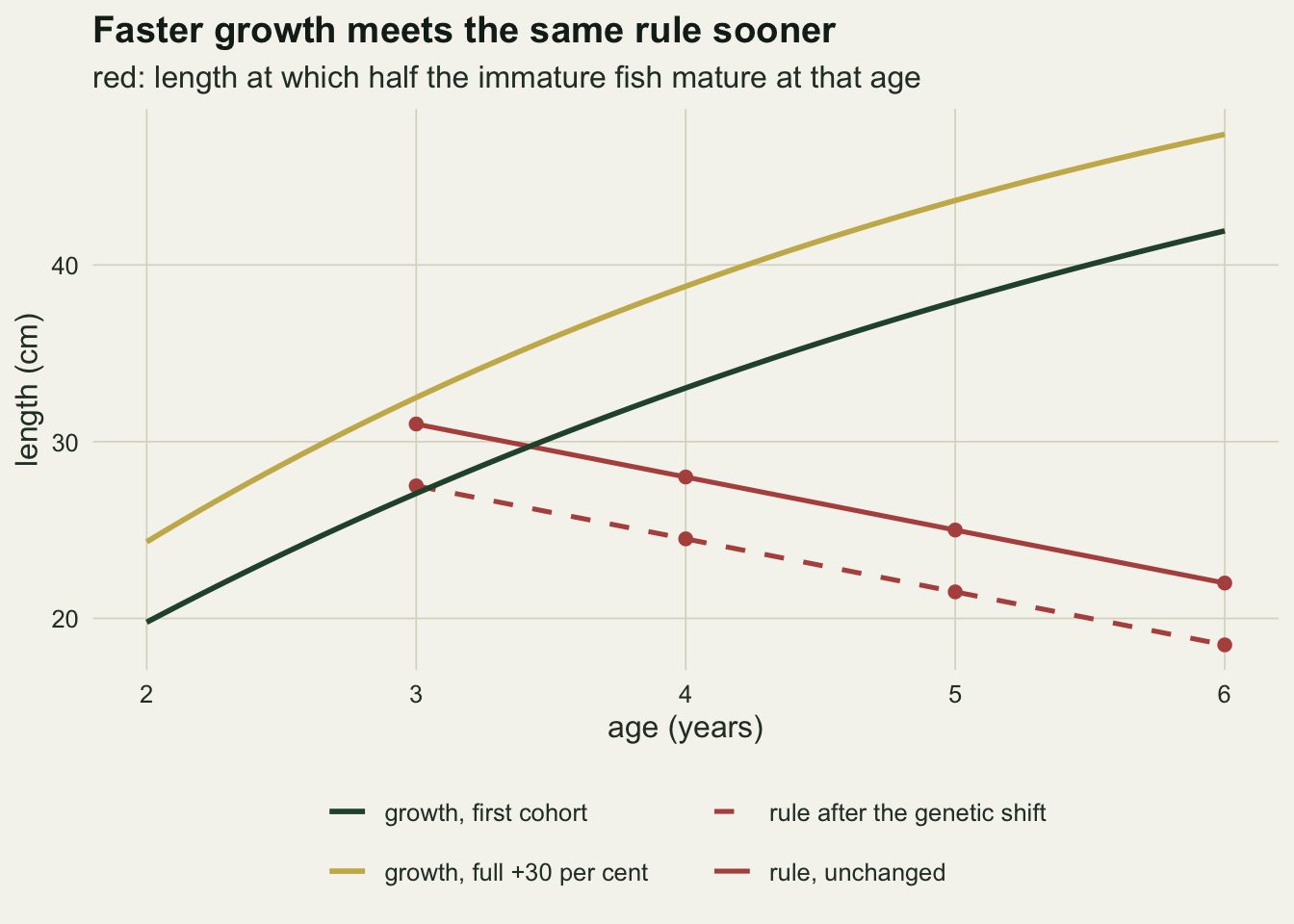
Twenty-five years of survey, read two ways
Each cell below is 200 simulated 25-year survey series. A summary counts as reporting earlier maturation when its yearly values have a negative least squares slope on year with a p-value below 0.05. The table gives the share of series in which that happens, the median slope over the 200 series, and, for the PMRN, the share of survey years whose midpoint was undefined. Fish per age means fish per age class per survey year, so a series at 100 fish per age holds 2500 fish of each age over its 25 years.
n_ser <- 200
run_cell <- function(n_fish, scen, reps = n_ser) {
  out <- replicate(reps, sim_series(n_fish, scen))
  lp_rows <- n_head + n_year + seq_along(yr_p)
  list(a50_det = mean(out["a50_det", ]), a50_slope = median(out["a50_slope", ]),
       lp_det = mean(out["lp_det", ]), lp_slope = median(out["lp_slope", ]),
       lp_mean_slope = mean(out["lp_slope", ]), lp_sd = sd(out["lp_slope", ]),
       lp_q = quantile(out["lp_slope", ], c(0.25, 0.75)),
       lp_na = mean(out["lp_na", ]) / length(yr_p),
       a50_sep = mean(out["a50_sep", ]) / n_year,
       og_sep = mean(out["og_sep", ]) / (2 * n_year),
       lp_any_na = mean(out["lp_na", ] > 0),
       lp_wild = mean(out[lp_rows, ] > 40, na.rm = TRUE),
       lp_bias = apply(out[lp_rows, , drop = FALSE], 1, median, na.rm = TRUE) - true_lp)
}
mc_se_max <- sqrt(0.25 / n_ser)

set.seed(2002)
main_grid <- expand.grid(scen = c("none", "grow15", "grow30", "genetic"),
                         n_fish = c(100, 400), stringsAsFactors = FALSE)
main_res <- lapply(seq_len(nrow(main_grid)),
                   function(i) run_cell(main_grid$n_fish[i], main_grid$scen[i]))
pick <- function(field) vapply(main_res, function(r) r[[field]], 0)
main_tab <- data.frame(main_grid, a50_det = pick("a50_det"), a50_slope = pick("a50_slope"),
                       lp_det = pick("lp_det"), lp_slope = pick("lp_slope"),
                       lp_na = pick("lp_na"), lp_any_na = pick("lp_any_na"),
                       a50_sep = pick("a50_sep"), og_sep = pick("og_sep"))
sep_a50_max <- max(main_tab$a50_sep)
sep_og_max  <- max(main_tab$og_sep)
sep_og_cell <- main_tab[which.max(main_tab$og_sep), ]
scen_lab <- c(none = "no change", grow15 = "growth +15 per cent",
              grow30 = "growth +30 per cent", genetic = "rule shift 3.5 cm")
sep_og_lab <- scen_lab[[sep_og_cell$scen]]
grow_rows <- main_tab$scen %in% c("grow15", "grow30")
n_grow_det <- sum(round(main_tab$a50_det[grow_rows] * n_ser))
n_grow_all <- sum(grow_rows) * n_ser
cell <- function(scen, n_fish) main_tab[main_tab$scen == scen & main_tab$n_fish == n_fish, ]
g30_100 <- cell("grow30", 100); g30_400 <- cell("grow30", 400)
g15_100 <- cell("grow15", 100); g15_400 <- cell("grow15", 400)
gen_100 <- cell("genetic", 100); gen_400 <- cell("genetic", 400)
non_100 <- cell("none", 100); non_400 <- cell("none", 400)
na_100_rng <- range(main_tab$lp_na[main_tab$n_fish == 100])| scenario | fish per age | A50 detects | A50 slope (yr/yr) | PMRN detects | PMRN slope (cm/yr) | undefined years | series with any undefined year |
|---|---|---|---|---|---|---|---|
| no change | 100 | 0.030 | 0.0000 | 0.025 | 0.004 | 0.095 | 0.905 |
| growth +15 per cent | 100 | 1.000 | -0.0123 | 0.015 | 0.013 | 0.076 | 0.855 |
| growth +30 per cent | 100 | 1.000 | -0.0214 | 0.000 | 0.035 | 0.078 | 0.885 |
| rule shift 3.5 cm | 100 | 1.000 | -0.0146 | 0.585 | -0.119 | 0.089 | 0.880 |
| no change | 400 | 0.020 | -0.0001 | 0.040 | 0.002 | 0.003 | 0.070 |
| growth +15 per cent | 400 | 1.000 | -0.0122 | 0.030 | 0.003 | 0.002 | 0.045 |
| growth +30 per cent | 400 | 1.000 | -0.0217 | 0.030 | 0.014 | 0.002 | 0.055 |
| rule shift 3.5 cm | 400 | 1.000 | -0.0146 | 1.000 | -0.133 | 0.002 | 0.050 |
The A50 reports earlier maturation in 1.000 of the series with 30 per cent faster growth at 100 fish per age and in 1.000 of those with 15 per cent faster growth, where the maturation rule never changed. Its median slopes, -0.0214 and -0.0123 years per year, sit on the infinite-survey values derived above. Nothing about that is a sampling failure: the A50 is doing what it is defined to do, which is to report when fish are mature, and they are mature earlier. With no change at all it reports a fall in 0.030 of series at 100 fish per age and 0.020 at 400, close to the one-sided rate of 0.025 that a two-sided test at 0.05 puts in each tail.
The PMRN midpoint reports a fall in 0.000 of the 30 per cent growth series at 100 fish per age and 0.030 at 400, and in 0.015 and 0.030 under 15 per cent growth; with no change, 0.025 and 0.040. The Monte Carlo standard error of any share in the table is at most 0.035. Its median slope under growth is +0.035 cm per year at 100 fish per age and +0.014 at 400. That residual slope belongs to this generator, including its sign; it is not a property of the PMRN in general and is not read as one here. Nor is it only a small-sample effect. An infinitely large survey already reads a slope of +0.0188 cm per year under 30 per cent faster growth and +0.0065 under 15 per cent, because the age-4 ogive mixes fish that matured at 3 and fish that matured at 4 and is not logistic in length. A logistic curve fitted to it misses in the lower tail, which is where the midpoint is, and faster growth pushes the midpoint further into that tail. The mean-increment approximation adds only the near-constant offset derived above.
Under the genetic shift both summaries move. The A50 falls in 1.000 of series with a median slope of -0.0146 years per year. The PMRN finds the change in 1.000 of series at 400 fish per age, with a median slope of -0.133 cm per year against the target of -0.136. At 100 fish per age it finds it in only 0.585, and its median slope is -0.119.
The last two columns show a cost that has nothing to do with the shift. At 100 fish per age, between 0.076 and 0.095 of the survey years had no midpoint in the bracket in every scenario, 0.089 under the genetic shift, and 0.880 of the genetic series lost at least one year that way; at 400 fish per age the genetic shares are 0.002 and 0.050. A trend regression that drops those years silently is fitted to fewer points than the report implies. A related case is separation, where every immature fish in a sample is shorter or younger than every mature one and the logistic fit has no finite maximum; glm() warns and returns a steep curve, and the fits here do the same. It was rare: at most 0.9 per cent of the yearly A50 fits in any cell, and at most 0.7 per cent of the length ogives, in the cell with 100 fish per age and growth +30 per cent.
set.seed(1861)
one_grow <- sim_series(100, "grow30")
one_gene <- sim_series(100, "genetic")
series_df <- function(v, lab) {
  rbind(data.frame(year = seq_len(n_year), value = v[n_head + seq_len(n_year)],
                   summary = "A50 (years)", scenario = lab),
        data.frame(year = yr_p, value = v[n_head + n_year + seq_along(yr_p)],
                   summary = "midpoint, age 4 (cm)", scenario = lab))
}
ser_df <- rbind(series_df(one_grow, "growth +30 per cent, rule unchanged"),
                series_df(one_gene, "rule shift 3.5 cm, growth unchanged"))
truth_df <- rbind(
  data.frame(year = yr_p, value = true_lp, summary = "midpoint, age 4 (cm)",
             scenario = "rule shift 3.5 cm, growth unchanged"),
  data.frame(year = yr_p, value = mid4, summary = "midpoint, age 4 (cm)",
             scenario = "growth +30 per cent, rule unchanged"))
n_gap_grow <- sum(is.na(one_grow[n_head + n_year + seq_along(yr_p)]))
n_gap_gene <- sum(is.na(one_gene[n_head + n_year + seq_along(yr_p)]))

ggplot(ser_df, aes(year, value)) +
  geom_line(data = truth_df, colour = te_rust, linetype = "dashed", linewidth = 0.7) +
  geom_smooth(method = "lm", formula = y ~ x, se = FALSE,
              colour = te_gold, linewidth = 0.9, na.rm = TRUE) +
  geom_point(colour = te_forest, size = 1.8, na.rm = TRUE) +
  facet_grid(summary ~ scenario, scales = "free_y") +
  labs(x = "survey year", y = NULL,
       title = "The A50 falls in both; the midpoint falls in one",
       subtitle = "gold: least squares trend; dashed red: the true midpoint") +
  theme_datasheet()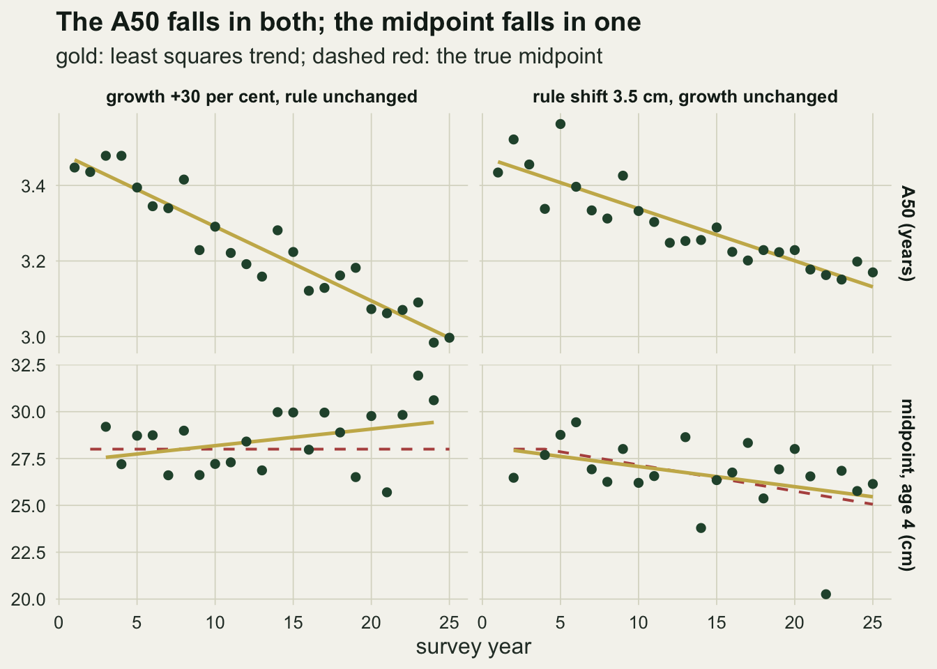
In the two series drawn for the figure, 2 and 2 of the 24 PMRN years were undefined and appear as gaps.
What the PMRN costs: power and a shallower slope
The genetic cell was run at two further survey sizes, 50 and 200 fish per age, to draw the cost as a curve rather than two points.
set.seed(2004)
extra_res <- lapply(c(50, 200), function(n_f) run_cell(n_f, "genetic"))
gen_res  <- list(extra_res[[1]], main_res[[which(main_grid$scen == "genetic" & main_grid$n_fish == 100)]],
                 extra_res[[2]], main_res[[which(main_grid$scen == "genetic" & main_grid$n_fish == 400)]])
pow_tab <- data.frame(n_fish = c(50, 100, 200, 400),
                      power = vapply(gen_res, function(r) r$lp_det, 0),
                      slope = vapply(gen_res, function(r) r$lp_slope, 0),
                      slope_mean = vapply(gen_res, function(r) r$lp_mean_slope, 0),
                      slope_se = 1.2533 * vapply(gen_res, function(r) r$lp_sd, 0) / sqrt(n_ser),
                      q1 = vapply(gen_res, function(r) r$lp_q[[1]], 0),
                      q3 = vapply(gen_res, function(r) r$lp_q[[2]], 0),
                      na_share = vapply(gen_res, function(r) r$lp_na, 0))
pow_tab$power_se <- sqrt(pow_tab$power * (1 - pow_tab$power) / n_ser)
pow_tab$shallow  <- 1 - pow_tab$slope / true_slope
pow_tab$shallow_mean <- 1 - pow_tab$slope_mean / true_slope
row_of <- function(n_f) pow_tab[pow_tab$n_fish == n_f, ]
p50 <- row_of(50); p100 <- row_of(100); p200 <- row_of(200); p400 <- row_of(400)
At 50 fish per age the PMRN finds the genetic shift in 0.185 of series, at 100 in 0.585, at 200 in 0.935 and at 400 in 1.000, each with a Monte Carlo standard error of at most 0.035. A programme sampling 100 fish of each age every year for 25 years would miss a real change in its maturation rule in 42 of 100 such surveys.
The slope is also flattened, and the flattening grows as the sample shrinks. Against the target of -0.136 cm per year, the median estimated slope is -0.133 at 400 fish per age, -0.132 at 200, -0.119 at 100 and -0.066 at 50: shallower by 2, 3, 13 and 52 per cent. The mean slope, which feels the long tail of wild series, is shallower still: -0.113 at 100 fish per age, 17 per cent below the target. Not all of that is a small-sample cost. The same estimator in an infinitely large survey, computed from the exact proportions earlier, reads the slope at -0.128, 6 per cent shallower than the target (the dotted gold line in the right panel), so that part of the flattening does not shrink with survey size: it is the limit a larger and larger survey approaches. At 100 fish per age the PMRN misses the change in a large share of series and its typical slope lies above that limit as well. At 400 fish per age the power cost has gone, and the median slope lies between that limit and the target, -0.005 cm per year from the limit against a Monte Carlo standard error of 0.002. At that size the small-sample error is small, and in the median slope it runs the other way from the shape error, so the two partly cancel. An infinitely large survey would read the slope at -0.128.
pow_plot <- ggplot(pow_tab, aes(n_fish, power)) +
  geom_errorbar(aes(ymin = power - 1.96 * power_se, ymax = power + 1.96 * power_se),
                width = 0.04, colour = te_ink, linewidth = 0.5) +
  geom_line(colour = te_forest, linewidth = 0.9) +
  geom_point(colour = te_forest, size = 2.4) +
  scale_x_log10(breaks = pow_tab$n_fish) +
  scale_y_continuous(limits = c(0, 1)) +
  labs(x = "fish per age per year", y = "share of series detecting the shift",
       title = "Power") +
  theme_datasheet()
slope_plot <- ggplot(pow_tab, aes(n_fish, slope)) +
  geom_hline(yintercept = true_slope, linetype = "dashed", colour = te_rust, linewidth = 0.7) +
  geom_hline(yintercept = inf_slope[["genetic"]], linetype = "dotted", colour = te_gold,
             linewidth = 0.9) +
  geom_errorbar(aes(ymin = q1, ymax = q3), width = 0.04, colour = te_ink, linewidth = 0.5) +
  geom_line(colour = te_forest, linewidth = 0.9) +
  geom_point(colour = te_forest, size = 2.4) +
  scale_x_log10(breaks = pow_tab$n_fish) +
  labs(x = "fish per age per year", y = "PMRN slope (cm per year)",
       title = "Median slope",
       subtitle = "dashed red: true slope\ndotted gold: infinite survey") +
  theme_datasheet()
pow_plot + slope_plot + plot_annotation(theme = theme_datasheet())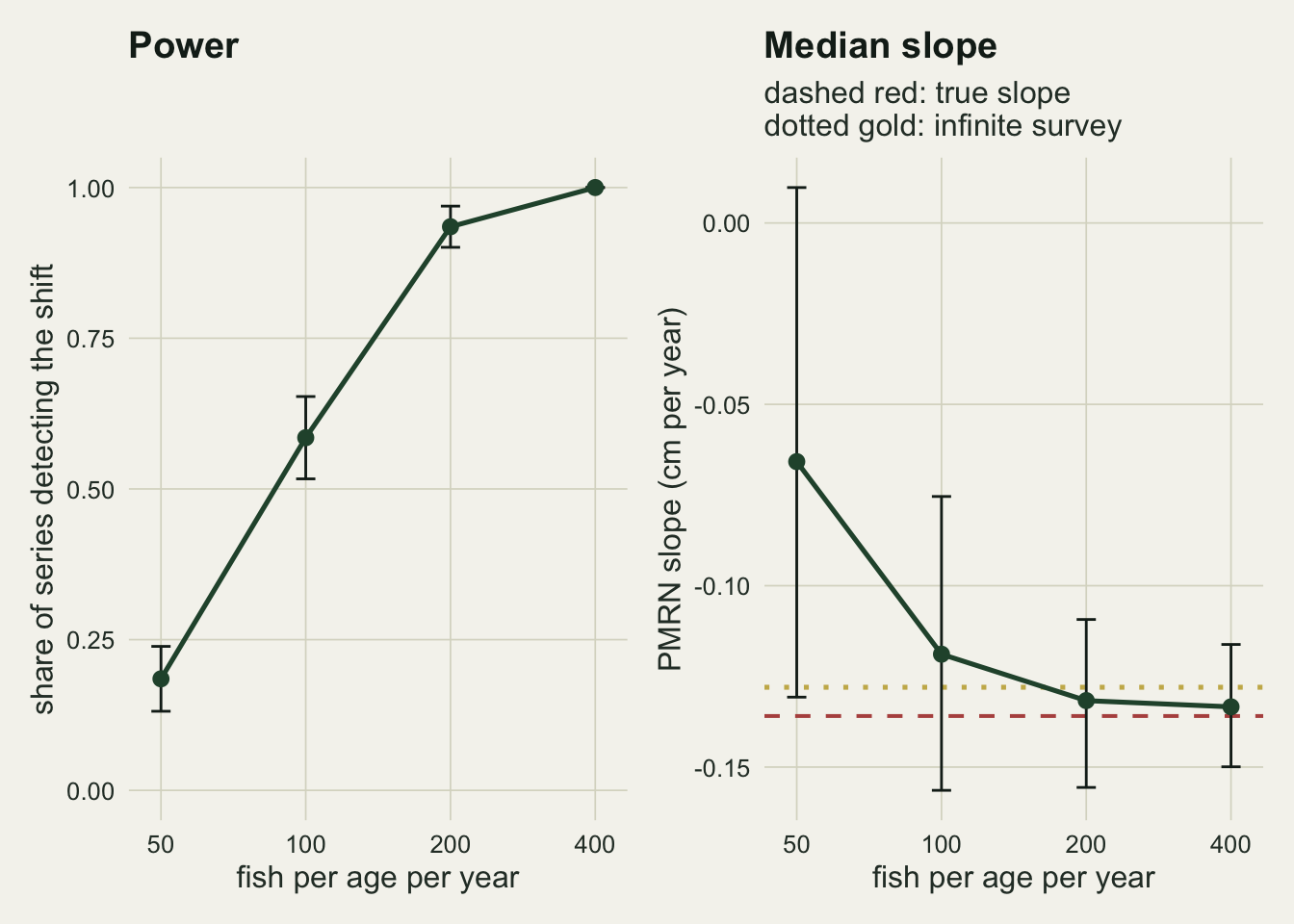
Where the flattening comes from
A least squares slope is not flattened by noise that is the same in every year; it is flattened when the error of the yearly estimate changes with the true value. Here that error has two parts: one would remain in an infinitely large survey, the other is the cost of a finite sample. The chunk below reads the median error of the estimated midpoint year by year in the genetic cells, sets it against the infinite-survey error from the exact chunk, splits the years into early and late halves, and then reruns the cell with one of the two ogives given more fish while the other stays at 100, to see which one carries the small-sample part.
bias_100 <- main_res[[which(main_grid$scen == "genetic" & main_grid$n_fish == 100)]]$lp_bias
bias_400 <- main_res[[which(main_grid$scen == "genetic" & main_grid$n_fish == 400)]]$lp_bias
early <- yr_p <= 13
bias_early_100 <- mean(bias_100[early]); bias_late_100 <- mean(bias_100[!early])
bias_early_400 <- mean(bias_400[early]); bias_late_400 <- mean(bias_400[!early])
inf_gen   <- inf_err[, "genetic"]
inf_early <- mean(inf_gen[early]); inf_late <- mean(inf_gen[!early])
fs_slope_100 <- yr_slope(bias_100 - inf_gen)
fs_slope_400 <- yr_slope(bias_400 - inf_gen)
gap_400      <- max(abs(bias_400 - inf_gen))
wild_100 <- main_res[[which(main_grid$scen == "genetic" & main_grid$n_fish == 100)]]$lp_wild
wild_400 <- main_res[[which(main_grid$scen == "genetic" & main_grid$n_fish == 400)]]$lp_wild
last_coh <- n_year - 4
imm4_first <- 100 * (1 - p_mature(4, 0, "genetic"))
imm4_last  <- 100 * (1 - p_mature(4, last_coh, "genetic"))
mat3_first <- 100 * p_mature(3, 0, "genetic")
mat3_last  <- 100 * p_mature(3, last_coh, "genetic")

set.seed(2007)
more_age3 <- run_cell(c(100, 400, 100, 100, 100), "genetic")
more_age4 <- run_cell(c(100, 100, 400, 100, 100), "genetic")
sd_len4 <- sd(l_inf * (1 - exp(-4 * k_nodes)))
z_start <- (mid4 - l4_start) / sd_len4
z_end   <- (lp_end - l4_start) / sd_len4
In the infinite survey the error of the midpoint is -0.065 cm in survey year 2 and +0.115 cm in year 25, the gold line in the figure below. The cause is the shape of the age-4 ogive. A fish mature at age 4 matured either at 3 or at 4, so the proportion mature at a given length at age 4 is one minus the product of two probabilities of staying immature, each logistic in its own length, and that is not a logistic curve in length at age 4. A logistic curve fitted to it follows the bulk of the fish and misses in the lower tail, and the midpoint sits in that tail: the mean length at age 4 at the starting growth rate is 33.0 cm with a spread of 3.2 cm from growth variation, so as the rule falls the midpoint moves from 1.6 to 2.5 standard deviations below the mean length, and the error rises with it. The measurement error is not the cause: without it the infinite-survey slope is -0.125, further from the target than the -0.128 with it. Nor is the mean increment, whose offset was near-constant.
At 100 fish per age the median error of the midpoint is +0.13 cm in survey years 2 to 13 and +0.41 cm in years 14 to 25; at 400 fish per age the two halves are -0.03 and +0.08, and in the infinite survey -0.05 and +0.05. The median is used because a few estimates lie far above the truth: 0.8 per cent of the defined midpoints at 100 fish per age lie above 40 cm, against 0.00 per cent at 400, and those points also pull on the least squares slopes. At 100 fish per age the yearly errors sit above the infinite-survey line in both halves and rise faster than it, by +0.0122 cm per year: that is the small-sample flattening. At 400 fish per age they stay within 0.23 cm of it in every year, and their trend relative to it, +0.0012 cm per year, is about a tenth of that.
The ogive swap says which sample carries the small-sample part. Giving the age-3 ogive 400 fish while the age-4 sample stays at 100 leaves the power at 0.610, with a median slope of -0.118; giving the age-4 ogive 400 fish instead lifts it to 1.000, with a slope of -0.130. The problem is the older ogive, not the younger one.
The exact proportions from the earlier chunk explain why. At age 4, 16.4 of every 100 fish of the first cohort are still immature, and in the last cohort the survey reaches, born in year 21, only 6.0 are. The lower tail of the age-4 ogive, where the midpoint sits, is placed by those few immature fish, and as the rule shifts down there are fewer of them. The age-3 ogive goes the other way: its share of mature fish rises from 21.4 to 41.1 per cent, so it gets better determined as the rule falls. In this generator, then, both parts of the flattening sit in the older ogive: the small-sample part comes from fitting it on a thinning set of immature fish, and the part that no survey size removes from fitting it with a logistic curve.
bias_df <- rbind(data.frame(year = yr_p, bias = bias_100, n_lab = "100 fish per age"),
                 data.frame(year = yr_p, bias = bias_400, n_lab = "400 fish per age"),
                 data.frame(year = yr_p, bias = inf_gen, n_lab = "infinite survey"))
ggplot(bias_df, aes(year, bias, colour = n_lab)) +
  geom_hline(yintercept = 0, colour = te_body, linewidth = 0.4) +
  geom_line(linewidth = 0.9) +
  geom_point(size = 1.9) +
  scale_colour_manual(values = c(te_rust, te_forest, te_gold), name = NULL) +
  labs(x = "survey year", y = "estimated minus true midpoint (cm)",
       title = "The error grows as the true midpoint falls",
       subtitle = "median over 200 series, and the exact infinite-survey error;\nthe true midpoint falls from year 5 on") +
  theme_datasheet() +
  theme(legend.position = "bottom")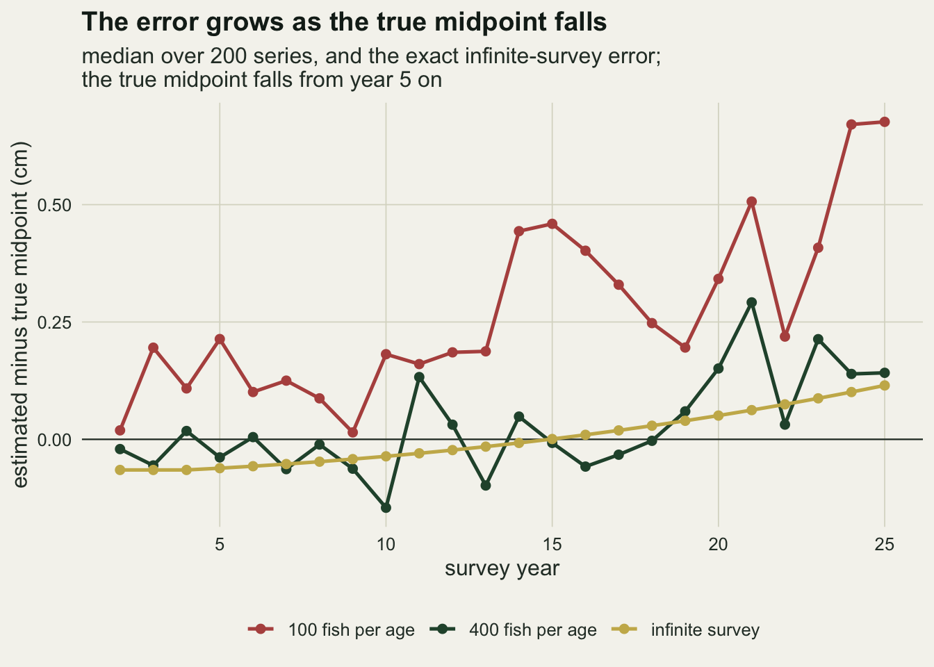
When plasticity acts outside length
Kraak pointed out in 2007 that the PMRN separates growth from evolution only when growth is the whole of the plastic response (her example was temperature, in North Sea plaice). If a fish in good condition matures at a smaller length than a fish of the same age and length in poor condition, then better feeding moves the norm itself, and the PMRN reads that plastic shift as evolution. The chunk below runs two versions of that case at 400 fish per age, the survey size at which the genetic shift was found in 1.000 of series. In both, cohort mean growth rises by 30 per cent and the rule’s intercept falls with growth, by 11.7 cm per unit of relative growth, so that the cohort-average rule ends 3.5 cm lower, as in the genetic scenario. In the first version the rule follows the cohort’s environment: every fish of a well-fed cohort matures at a smaller length, whatever its own growth. In the second it follows the individual: each fish’s intercept depends on its own growth coefficient.
n_kraak <- 100
set.seed(2027)
kr_env <- run_cell(400, "kraak_env", reps = n_kraak)
kr_ind <- run_cell(400, "kraak_ind", reps = n_kraak)
kr_se  <- sqrt(0.25 / n_kraak)
imm4_kraak <- 400 * (1 - p_mature(4, last_coh, "kraak_env"))
l4_kraak   <- l_inf * (1 - exp(-4 * k_start * k_mult(last_coh, "kraak_env")))
With the rule following the cohort’s environment, the PMRN reports earlier maturation in 0.48 of series, with a median slope of -0.095 cm per year, where the genetic shift of the same size gave 1.000 and -0.133. Nothing genetic happened, and in about half the series the PMRN reports evolution anyway. That it does so less often than for the genetic shift is not discrimination: it is the flattening mechanism again. Faster growth and a lower rule together leave only 2.9 immature fish in a sample of 400 at age 4 in the last cohort, whose mean length at age 4 is 38.0 cm, and the midpoint has to be extrapolated far below the fish. A reader who took the lower detection rate as evidence against evolution would be reading the estimator’s blind spot as biology.
The individual version is the less obvious half. There the PMRN reports a fall in 0.00 of series, with a median slope of +0.010, although the average rule fell by exactly as much. In this generator length at a given age is fixed by the growth coefficient, so a rule written on a fish’s own growth rate is a rule written on its length in disguise, and the PMRN absorbs it. Kraak’s case needs a cause that length at age does not carry, such as condition or an environment the whole cohort shares. Shares in this section carry a Monte Carlo standard error of at most 0.05.
What to report
Report the A50 as a description of when fish are mature, not as evidence about the maturation rule. In this simulation it reported earlier maturation in 800 of the 800 growth-only series, and that is its correct behaviour. If the question is whether the rule changed, the A50 cannot answer it, and a trend in it should be quoted next to a trend in length at age.
When a PMRN midpoint trend is reported, give the number of fish per age behind each ogive, and read the result against a power statement of the kind in the figure above. A non-significant PMRN trend from a survey of 100 fish per age says little: in this generator such a survey missed a shift of the rule by 3.5 cm over 25 cohorts, 2.94 cm of it inside the cohorts the survey sees at age 4, in 42 of 100 series. Where the survey design can be changed, extra fish help most at the older age of the ogive pair, where immature fish are scarce: in this generator 400 fish at age 4 with 100 at every other age gave a power of 1.000 and a median slope of -0.130, against 1.000 and -0.133 with 400 at every age.
Say how many years had no midpoint, and whether the trend regression dropped them. At 100 fish per age that was 9 per cent of years here. Report the number of immature fish in the sample at the older age of the pair and the range of their lengths, so a reader can see when the midpoint has been extrapolated below most of the fish.
State the plastic causes that length does not carry and what is known about them in the population, because those are the ones the PMRN will read as evolution.
Honest limits
The generator has no mortality and no fishing, and the survey draws its fish at random from each age. In a real stock, size-selective fishing and size-selective gear, of the kind in gill-net selectivity and the fish it cannot see, make the sampled fish at each age a non-random subset, and if maturity and size are linked that selection enters both ogives. Nothing here measures what that does to the midpoint.
Growth is deterministic given the growth coefficient: a fish’s length at every age follows from one number. That is why the PMRN absorbed the individual version of Kraak’s case, and it is not how fish grow. With variation in the asymptote, or year effects on growth, fish of the same length at age 4 differ in their history, the length at age 3 is not a fixed function of the length at age 4, and the mean-increment approximation in the demographic estimator carries more error than it does here.
The estimator is the simplest version of the demographic method: separate logistic fits at ages 3 and 4, one mean increment, one midpoint. The logistic ogive at age 4 is itself an approximation, and it is the source of the flattening that remains in an infinitely large survey. Applications often pool years or cohorts in one model with smooth terms, or use the whole age range; a smooth ogive is one answer to the shape error, and pooling trades bias for variance in ways this post does not measure. The bisection bracket from 15 to 50 cm is a choice; a wider bracket would define a midpoint in more years, and some of those midpoints would be extrapolations far outside the data.
The magnitudes are fixed design choices: 30 and 15 per cent faster growth, a 3.5 cm shift in the rule, a PMRN width of 2.5 cm. Power depends on all of them. A steeper norm or a larger shift would move the curve in the power figure, and so would reading the midpoint at an age where more fish are still immature, so it should be read as the shape of the cost, not as a sample size to copy.
The significance rule takes the two-sided p-value of an ordinary least squares slope over 24 or 25 yearly values treated as independent, and counts only negative slopes. In this generator every year’s samples are fresh, independent draws, so that assumption holds by design and the rates under no change were 0.020 to 0.040 against a nominal 0.025. In a real survey, year effects on catchability or growth and serial correlation between years break the assumption, and a check like that one does not carry over.
References
Heino M, Dieckmann U, Godo OR 2002 Evolution 56(4):669-678 (10.1111/j.0014-3820.2002.tb01378.x)
Olsen EM, Heino M, Lilly GR, Morgan MJ, Brattey J, Ernande B, Dieckmann U 2004 Nature 428(6986):932-935 (10.1038/nature02430)
Dieckmann U, Heino M 2007 Marine Ecology Progress Series 335:253-269 (10.3354/meps335253)
Kraak SBM 2007 Marine Ecology Progress Series 335:295-300 (10.3354/meps335295)