library(ggplot2)
library(patchwork)

te_paper  <- "#f5f4ee"
te_ink    <- "#16241d"
te_body   <- "#2c3a31"
te_forest <- "#275139"
te_rust   <- "#b5534e"
te_gold   <- "#c9b458"
te_line   <- "#dad9ca"

theme_datasheet <- function() {
  theme_minimal(base_size = 12) +
    theme(plot.background  = element_rect(fill = te_paper, colour = NA),
          panel.background = element_rect(fill = te_paper, colour = NA),
          panel.grid.major = element_line(colour = te_line, linewidth = 0.3),
          panel.grid.minor = element_blank(),
          text             = element_text(colour = te_body),
          plot.title       = element_text(colour = te_ink, face = "bold"),
          plot.subtitle    = element_text(colour = te_body),
          axis.text        = element_text(colour = te_body))
}Growth from tag-recapture increments
R
growth
fisheries
capture-recapture
measurement error
nonlinear regression
simulation
ecology tutorial
Fabens fits to tag-recapture increments do not estimate the length-at-age curve. Measuring in R how asymptote spread and length error bias Linf and K.
A lake zander programme has tagged fish for three seasons. Every fish caught in a fyke net is measured, given a numbered tag and put back; when a tagged fish turns up again, somebody measures it a second time and writes down how many days it was free. Nobody knows how old any of the fish are. What the programme has is a list of pairs of lengths and the time between them, and what the management plan wants is a von Bertalanffy curve: an asymptotic length and a growth coefficient to plug into a yield-per-recruit model built, like most such models, on length at age.
The standard route from increments to that curve rewrites the von Bertalanffy equation for increments. If each fish followed the population curve, its increment over a time at liberty would be the distance still to grow, times the fraction of that distance covered in the time: the increment equals the asymptote minus the release length, times one minus the exponential of minus the growth coefficient times the time at liberty. Age cancels out, so the two parameters can be fitted by nonlinear least squares with no ages at all. This is the Fabens form of the von Bertalanffy increment equation, the conventional tagging method whose asymptote Francis 1988 examined.
This site already fits growth curves, but always to length at known age. Fitting growth curves with nls simulates lengths at known ages and compares the Ford-Walford plot with a direct nls fit. Individual growth curves with nlme gives every fish its own asymptote and growth coefficient and fits them with a mixed model, and its honest limits say plainly that tagged-fish increments at unknown age were not simulated there. This post simulates that data type. The problem is not new. Sainsbury 1980 showed that individual variation in the growth parameters biases estimates of the growth coefficient downward; Francis 1988 argued that the asymptote from tagging data and the asymptote from age-length data are different quantities that should not be compared as if they were one; and Wang, Thomas and Somers 1995 built a likelihood around the fact that a fish’s release length carries information about its own asymptote, which is the source of the larger bias measured below. What follows demonstrates that bias on simulated fish, adds the second source, measurement error in the release length, and checks the size of each effect against a large-sample expression. The measurement-error part is the errors-in-variables problem from measurement error and regression dilution, with one twist: here it does not attenuate the slope, it steepens it.
Tagged fish with no ages
Each simulated fish has its own asymptote, drawn from a normal distribution around a population mean of 60 cm, and all fish share a growth coefficient of 0.30 per year with the curve starting at zero length at age zero. A fish is tagged at an age drawn from one of three distributions between half a year and six years, stays free for a time drawn uniformly between 0.3 and 2 years, and is measured at release and at recapture with independent normal error. The population mean curve, the one a length-at-age study estimates, has exactly the generating parameters, because the asymptote enters the curve linearly.
mu_set  <- 60       # population mean asymptote, cm
K_set   <- 0.30     # growth coefficient, per year
n_fish  <- 300      # recaptured fish per data set
n_rep   <- 300      # data sets per cell, fixed before any result was seen
age_lev <- c("uniform", "young-skewed", "old-skewed")

draw_age <- function(n, shape) switch(shape,
  "uniform"      = runif(n, 0.5, 6),
  "young-skewed" = 0.5 + 5.5 * rbeta(n, 1, 3),
  "old-skewed"   = 0.5 + 5.5 * rbeta(n, 3, 1),
  "lognormal"    = pmin(rlnorm(n, log(2), 0.5), 15))

tag_fish <- function(n, sd_linf, sd_meas, shape = "uniform",
                     liberty = c(0.3, 2), sd_k = 0) {
  linf_i <- rnorm(n, mu_set, sd_linf)
  k_i    <- K_set * exp(rnorm(n, 0, sd_k) - sd_k^2 / 2)   # mean K_set
  age1   <- draw_age(n, shape)
  at_lib <- runif(n, liberty[1], liberty[2])
  len1 <- linf_i * (1 - exp(-k_i * age1))
  len2 <- linf_i * (1 - exp(-k_i * (age1 + at_lib)))
  data.frame(age1 = age1, at_lib = at_lib,
             len1 = len1 + rnorm(n, 0, sd_meas),
             len2 = len2 + rnorm(n, 0, sd_meas))
}
The Fabens model is linear in the asymptote once the growth coefficient is fixed, so the least squares fit can profile the asymptote out and search one dimension for the growth coefficient. That gives the same answer as nls, needs no starting values, and does not fail on data with no scatter at all, which nls does. The standard errors come from the same Gauss-Newton approximation that nls prints. The length-at-age reference uses the same trick on release length against the true release age, which a real tagging study would not have.
vb_profile <- function(y, x_len, h) {   # y = (Linf - x_len) * h
  lin <- sum(h * (y + x_len * h)) / sum(h^2)
  list(linf = lin, rss = sum((y - (lin - x_len) * h)^2))
}
fit_fabens <- function(len1, len2, at_lib) {
  inc <- len2 - len1
  k_hat <- optimize(function(k) vb_profile(inc, len1, 1 - exp(-k * at_lib))$rss,
                    c(0.01, 3), tol = 1e-9)$minimum
  hh <- 1 - exp(-k_hat * at_lib)
  pr <- vb_profile(inc, len1, hh)
  jac <- cbind(hh, (pr$linf - len1) * at_lib * exp(-k_hat * at_lib))
  vc  <- pr$rss / (length(inc) - 2) * solve(crossprod(jac))
  c(linf = pr$linf, k = k_hat, se_linf = sqrt(vc[1, 1]), se_k = sqrt(vc[2, 2]))
}
fit_age_length <- function(age, len) {
  k_hat <- optimize(function(k) vb_profile(len, 0, 1 - exp(-k * age))$rss,
                    c(0.01, 3), tol = 1e-9)$minimum
  c(linf = vb_profile(len, 0, 1 - exp(-k_hat * age))$linf, k = k_hat)
}

set.seed(4107)
fish <- tag_fish(n_fish, sd_linf = 6, sd_meas = 2)
fb_one <- fit_fabens(fish$len1, fish$len2, fish$at_lib)
nls_one <- nls(I(len2 - len1) ~ (Linf - len1) * (1 - exp(-K * at_lib)),
               data = fish, start = list(Linf = 60, K = 0.3))
gap_nls <- max(abs(c(coef(nls_one), summary(nls_one)$coefficients[, 2]) - fb_one))
al_one <- fit_age_length(fish$age1, fish$len1)
One data set of 300 recaptured fish, with an among-fish standard deviation of the asymptote of 6 cm (ten per cent of the mean) and a measurement error of 2 cm on each length. The profiled fit and nls agree to 7.4e-06 on both estimates and both standard errors. The Fabens fit returns an asymptote of 60.5 cm (standard error 1.3) and a growth coefficient of 0.287 (standard error 0.017). The same fish fitted on length at their true release ages give 61.7 cm and 0.288. In the figure below the Fabens line and the population curve almost coincide. A single data set cannot say whether that is because the method works or because two errors happen to cancel; that needs replication, and it needs the two sources of error taken one at a time.
fish$rate <- (fish$len2 - fish$len1) / fish$at_lib
len_seq <- seq(0, 70, by = 0.5)
lines_one <- rbind(
  data.frame(len1 = len_seq, rate = (mu_set - len_seq) * mean((1 - exp(-K_set * fish$at_lib)) / fish$at_lib),
             curve = "population curve"),
  data.frame(len1 = len_seq, rate = (fb_one["linf"] - len_seq) * mean((1 - exp(-fb_one["k"] * fish$at_lib)) / fish$at_lib),
             curve = "Fabens fit"))
ggplot(fish, aes(len1, rate)) +
  geom_hline(yintercept = 0, colour = te_line, linewidth = 0.6) +
  geom_point(colour = te_body, alpha = 0.45, size = 1.4) +
  geom_line(data = lines_one, aes(colour = curve), linewidth = 1) +
  scale_colour_manual(values = c("population curve" = te_forest, "Fabens fit" = te_rust),
                      name = NULL) +
  coord_cartesian(xlim = c(0, 70)) +
  labs(x = "length at release (cm)", y = "growth per year at liberty (cm)",
       title = "What a tagging study sees",
       subtitle = "lines: expected growth per year at liberty, averaged over the sampled times at liberty") +
  theme_datasheet() + theme(legend.position = "bottom")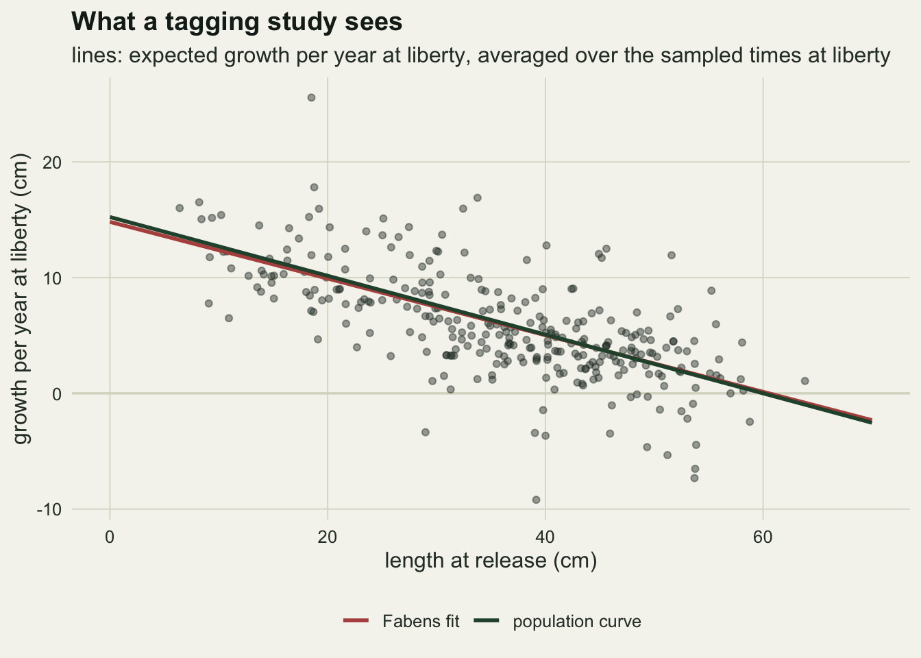
Where the least squares fit converges
Before any simulation it helps to know what the Fabens fit is aiming at when the sample is very large. For a single time at liberty the Fabens model is a straight line: the increment is a constant times the asymptote, minus the same constant times the release length. The least squares slope converges to the covariance of increment and observed release length divided by the variance of observed release length, and both moments can be written down.
Write \(h = 1 - e^{-K\Delta t}\) for the true fraction grown, \(\sigma^2\) for the measurement error variance and \(L_1\) for the true release length. Each fish’s increment is exactly \(h(L_{\infty,i} - L_1)\), so
\[ h^* = \frac{h\,[\operatorname{Var}(L_1) - \operatorname{Cov}(L_{\infty,i}, L_1)] + \sigma^2}{\operatorname{Var}(L_1) + \sigma^2}, \qquad K^* = -\frac{\log(1 - h^*)}{\Delta t}, \qquad L_\infty^* = \operatorname{E}L_1 + \frac{h\,(\mu - \operatorname{E}L_1)}{h^*}. \]
Both errors are visible in \(h^*\). Among fish of the same release length, the ones still growing fast tend to be the ones with the larger asymptote, so the covariance term flattens the line: \(h^*\) falls below \(h\), the growth coefficient is underestimated and the asymptote, where the line crosses zero growth, moves out. Measurement error in the release length enters twice: it inflates the variance of the predictor, as in ordinary regression dilution, but the same error also appears with the opposite sign in the increment, because the increment is recapture length minus release length. That shared error adds \(\sigma^2\) to the numerator and makes the line steeper, not flatter. This expression is derived here for the uniform release-age distribution by computing the two moments of \(1 - e^{-Ka}\); it is a check on the simulation, not a formula from the cited papers.
limit_fabens <- function(sd_linf, sd_meas, lib = 1, a_lo = 0.5, a_hi = 6,
                         k = K_set, mu = mu_set) {
  e1 <- (exp(-k * a_lo) - exp(-k * a_hi)) / (k * (a_hi - a_lo))
  e2 <- (exp(-2 * k * a_lo) - exp(-2 * k * a_hi)) / (2 * k * (a_hi - a_lo))
  g1 <- 1 - e1; g2 <- 1 - 2 * e1 + e2          # E(g) and E(g^2), g = 1 - exp(-k a)
  var_l1 <- (sd_linf^2 + mu^2) * g2 - mu^2 * g1^2
  cov_linf_l1 <- sd_linf^2 * g1
  h <- 1 - exp(-k * lib)
  h_star <- (h * (var_l1 - cov_linf_l1) + sd_meas^2) / (var_l1 + sd_meas^2)
  c(linf = mu * g1 + h * mu * (1 - g1) / h_star, k = -log(1 - h_star) / lib)
}
n_big <- 200000
set.seed(5310)
lim_grid <- expand.grid(sd_linf = c(0, 3, 6, 9), sd_meas = c(0, 2))
lim_tab <- do.call(rbind, lapply(seq_len(nrow(lim_grid)), function(j) {
  d <- tag_fish(n_big, lim_grid$sd_linf[j], lim_grid$sd_meas[j], liberty = c(1, 1))
  sim <- fit_fabens(d$len1, d$len2, d$at_lib)
  th  <- limit_fabens(lim_grid$sd_linf[j], lim_grid$sd_meas[j])
  data.frame(lim_grid[j, ], linf_sim = sim[["linf"]], k_sim = sim[["k"]],
             linf_lim = th[["linf"]], k_lim = th[["k"]])
}))
gap_lim_linf <- max(abs(lim_tab$linf_sim - lim_tab$linf_lim))
gap_lim_k <- max(abs(lim_tab$k_sim - lim_tab$k_lim))
lim_at <- function(sl, sm, what) lim_tab[lim_tab$sd_linf == sl & lim_tab$sd_meas == sm, what]
With one year at liberty for every fish and 200000 fish per fit, the simulated Fabens estimates match the expression to within 0.08 cm on the asymptote and 0.0010 on the growth coefficient across the eight cells. The limit with an asymptote spread of 6 cm and no measurement error is 64.0 cm and 0.253; with no spread and 2 cm of error it is 58.1 cm and 0.328; with both it is 61.6 cm and 0.279. These are not small-sample problems. More fish take the Fabens fit closer to these numbers, not closer to 60 cm and 0.30.
lim_long <- rbind(
  data.frame(sd_linf = lim_tab$sd_linf, sd_meas = lim_tab$sd_meas, par = "asymptote (cm)",
             limit = lim_tab$linf_lim, sim = lim_tab$linf_sim, truth = mu_set),
  data.frame(sd_linf = lim_tab$sd_linf, sd_meas = lim_tab$sd_meas, par = "growth coefficient (per year)",
             limit = lim_tab$k_lim, sim = lim_tab$k_sim, truth = K_set))
lim_long$error <- factor(sprintf("measurement SD %g cm", lim_long$sd_meas))
sd_fine <- seq(0, 9, by = 0.25)
lim_curve <- do.call(rbind, lapply(c(0, 2), function(sm) {
  th <- t(vapply(sd_fine, function(s) limit_fabens(s, sm), numeric(2)))
  rbind(data.frame(sd_linf = sd_fine, par = "asymptote (cm)", limit = th[, 1],
                   error = sprintf("measurement SD %g cm", sm)),
        data.frame(sd_linf = sd_fine, par = "growth coefficient (per year)", limit = th[, 2],
                   error = sprintf("measurement SD %g cm", sm)))
}))
ggplot(lim_long, aes(sd_linf, colour = error)) +
  geom_hline(aes(yintercept = truth), colour = te_body, linetype = "dashed", linewidth = 0.5) +
  geom_line(data = lim_curve, aes(y = limit), linewidth = 0.9) +
  geom_point(aes(y = sim), shape = 21, fill = te_paper, size = 2.6, stroke = 0.9) +
  facet_wrap(~ par, scales = "free_y") +
  scale_colour_manual(values = c(te_forest, te_rust), name = NULL) +
  labs(x = "among-fish SD of the asymptote (cm)", y = "Fabens estimate",
       title = "Where the Fabens fit converges",
       subtitle = "dashed line: the length-at-age parameter") +
  theme_datasheet() + theme(legend.position = "bottom")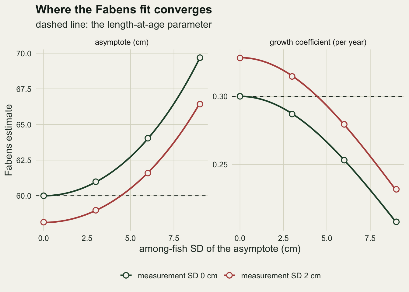
Two errors pulling opposite ways
The limit expression is for a single time at liberty and one release-age distribution. The realistic question is what a study of 300 fish with mixed times at liberty gets, and how much that depends on which fish were tagged. The grid crosses four values of the asymptote spread with four values of the measurement error and three release-age distributions: uniform between half a year and six years, skewed towards young fish, and skewed towards old fish. Tagging programmes catch what their gear selects, so tagged ages usually rise to a mode a year or two after recruitment and tail off with age. Of the sets used in this post the lognormal one added later in the post is the closest to that; young-skewed exaggerates the share of the youngest fish, and old-skewed is an extreme case included to show the range.
sd_linf_set <- c(0, 3, 6, 9); sd_meas_set <- c(0, 1, 2, 3)
cells <- expand.grid(sd_linf = sd_linf_set, sd_meas = sd_meas_set, shape = age_lev,
                     stringsAsFactors = FALSE)
set.seed(2290)
surf <- do.call(rbind, lapply(seq_len(nrow(cells)), function(j) {
  est <- t(replicate(n_rep, {
    d <- tag_fish(n_fish, cells$sd_linf[j], cells$sd_meas[j], cells$shape[j])
    fit_fabens(d$len1, d$len2, d$at_lib) }))
  data.frame(cells[j, ], linf = median(est[, 1]), k = median(est[, 2]),
             mcse_linf = 1.2533 * sd(est[, 1]) / sqrt(n_rep),
             cov_linf = mean(abs(est[, 1] - mu_set) <= qnorm(0.975) * est[, 3]),
             cov_k = mean(abs(est[, 2] - K_set) <= qnorm(0.975) * est[, 4]))
}))
sv <- function(sl, sm, shape, what) surf[surf$sd_linf == sl & surf$sd_meas == sm &
                                         surf$shape == shape, what]
mcse_max_u <- max(surf$mcse_linf[surf$shape != "old-skewed"])
free_cells <- surf[!(surf$sd_linf == 0 & surf$sd_meas == 0), ]
n_cov_ok <- sum(free_cells$cov_linf >= 0.9 & free_cells$cov_k >= 0.9)
With uniform release ages and no measurement error, an asymptote spread of 6 cm gives a median Fabens asymptote of 64.0 cm and growth coefficient of 0.250. With no spread and 2 cm of error the medians are 58.6 cm and 0.322, and with both 62.3 cm and 0.271. The directions are those of the limit expression and the sizes are similar to it. The Monte Carlo standard error of a median asymptote is at most 0.29 cm in the uniform and young-skewed cells, so none of these differences is noise.
The release-age distribution changes the size of both errors a great deal. Old fish are close to their own asymptote, so the differences in their release lengths reflect differences in asymptote more than differences in age. In the limit expression that makes the covariance term almost as large as the variance of release length, and the line flattens much further. With old-skewed tagging and a 6 cm spread without measurement error, the median asymptote is 74.7 cm and the growth coefficient 0.140; at a 9 cm spread they are 106.1 cm and 0.065. Young-skewed tagging gives 65.4 cm and 0.253 at a 6 cm spread, a little further out than the uniform case. Measurement error works the other way in all three panels: at 3 cm with no spread, the median asymptote is 57.2 cm for uniform ages, 54.7 cm for young-skewed and 55.1 cm for old-skewed, where the growth coefficient reaches 0.490.
surf$shape <- factor(surf$shape, levels = age_lev)
tile_plot <- function(col, truth, digits, ttl) {
  dd <- surf
  dd$rel <- 100 * (dd[[col]] / truth - 1)
  dd$fillv <- pmax(pmin(dd$rel, 30), -30)
  dd$lab <- sprintf(paste0("%.", digits, "f"), dd[[col]])
  ggplot(dd, aes(factor(sd_linf), factor(sd_meas), fill = fillv)) +
    geom_tile(colour = te_paper, linewidth = 0.8) +
    geom_text(aes(label = lab, colour = ifelse(abs(fillv) > 18, te_paper, te_ink)), size = 3.1) +
    scale_colour_identity() +
    facet_wrap(~ shape) +
    scale_fill_gradient2(low = te_forest, mid = te_paper, high = te_rust, midpoint = 0,
                         limits = c(-30, 30), name = "per cent\nfrom truth") +
    labs(x = "among-fish SD of the asymptote (cm)", y = "measurement SD (cm)", title = ttl) +
    theme_datasheet() + theme(panel.grid.major = element_blank())
}
tile_plot("linf", mu_set, 1, "Asymptote (truth 60 cm)") /
  tile_plot("k", K_set, 3, "Growth coefficient (truth 0.30)") +
  plot_annotation(theme = theme_datasheet())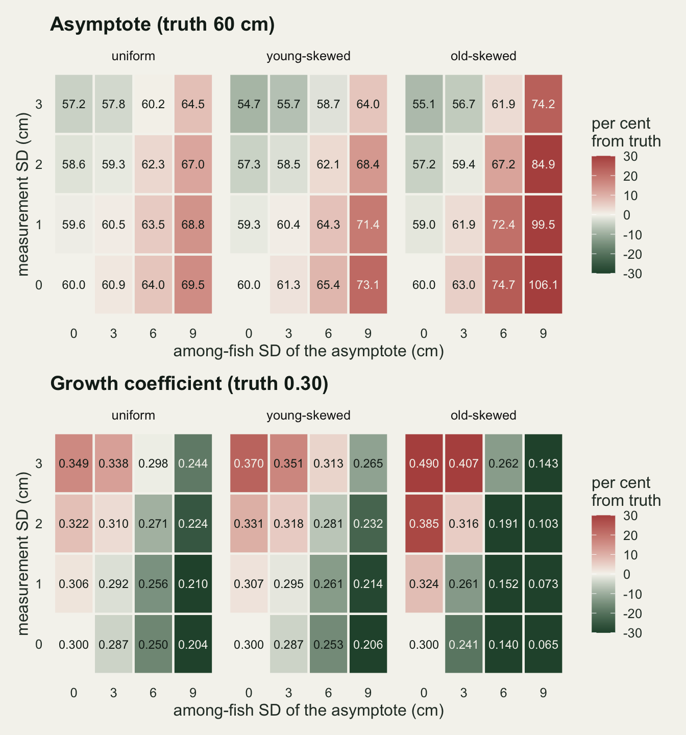
The pale diagonal in each panel is where the two errors cancel. It is not a property of the method; it is an accident of how much individual variation and how much measuring noise a particular population and a particular field crew happen to have. For uniform release ages the Fabens fit lands on 60.2 cm and 0.298 with a 6 cm spread and 3 cm of error, and the nominal 95 per cent intervals then cover both true values 95 and 96 per cent of the time. Move one cell to a 6 cm spread and 1 cm of error and the coverage is 15 and 7 per cent. Of the 45 cells with either source of error, 3 give at least 90 per cent coverage for both parameters. A well-behaved interval in a real study says nothing about which side of the diagonal the study is on.
Short liberty and a variable growth coefficient
Time at liberty sets how large the true increment is compared with the measuring error. Fish recaptured after a few weeks have grown a few millimetres, and the error in two length readings can be larger than that.
set.seed(6620)
lib_lev <- c("0.3 to 2 years", "0.1 to 0.5 years")
extra <- expand.grid(sd_meas = sd_meas_set, liberty = lib_lev, stringsAsFactors = FALSE)
ex_tab <- do.call(rbind, lapply(seq_len(nrow(extra)), function(j) {
  lib <- if (extra$liberty[j] == lib_lev[1]) c(0.3, 2) else c(0.1, 0.5)
  est <- t(replicate(n_rep, {
    d <- tag_fish(n_fish, 6, extra$sd_meas[j], liberty = lib)
    fit_fabens(d$len1, d$len2, d$at_lib) }))
  data.frame(extra[j, ], linf = median(est[, 1]), k = median(est[, 2]))
}))
ev <- function(sm, lb, what) ex_tab[ex_tab$sd_meas == sm & ex_tab$liberty == lib_lev[lb], what]
sd_k_set <- c(0, 0.1, 0.2)
set.seed(6621)
kv <- vapply(sd_k_set, function(sk) {
  est <- t(replicate(n_rep, { d <- tag_fish(n_fish, 6, 2, sd_k = sk)
                              fit_fabens(d$len1, d$len2, d$at_lib) }))
  c(median(est[, 1]), median(est[, 2]))
}, numeric(2))
With a 6 cm asymptote spread and uniform release ages, a study whose fish were free for between 0.1 and 0.5 years gets a median asymptote of 64.1 cm with perfect measuring, 57.6 cm with 2 cm of error and 52.6 cm with 3 cm, where the growth coefficient is 0.437. The same errors with 0.3 to 2 years at liberty give 64.0, 62.2 and 60.2 cm. With no error the time at liberty barely matters; with error, short liberty turns a moderate overestimate of the asymptote into a clear underestimate.
Individual variation in the growth coefficient, which Sainsbury 1980 treated together with variation in the asymptote, pushes in the same direction as the asymptote spread. Giving each fish a lognormal growth coefficient with the same mean and a log-scale standard deviation of 0.1 or 0.2, on top of the 6 cm asymptote spread and 2 cm error, moves the median asymptote from 62.2 cm to 62.7 and 63.8 cm, and the growth coefficient from 0.271 to 0.264 and 0.243 (with a variable growth coefficient the mean length-at-age curve is itself no longer exactly a von Bertalanffy curve with 60 cm and 0.30, so these are shifts, not biases against a fixed target). The two were drawn independently here; real fish that grow fast early often level off lower, and that correlation was not simulated.
ex_long <- rbind(
  data.frame(ex_tab[, c("sd_meas", "liberty")], par = "asymptote (cm)", est = ex_tab$linf, truth = mu_set),
  data.frame(ex_tab[, c("sd_meas", "liberty")], par = "growth coefficient (per year)", est = ex_tab$k, truth = K_set))
ex_long$liberty <- factor(ex_long$liberty, levels = lib_lev)
ggplot(ex_long, aes(sd_meas, est, colour = liberty)) +
  geom_hline(aes(yintercept = truth), colour = te_body, linetype = "dashed", linewidth = 0.5) +
  geom_line(linewidth = 0.9) + geom_point(size = 2.4) +
  facet_wrap(~ par, scales = "free_y") +
  scale_colour_manual(values = c(te_forest, te_rust), name = "time at liberty") +
  labs(x = "measurement SD of each length (cm)", y = "median Fabens estimate",
       title = "Short liberty hands the fit to the measuring error",
       subtitle = "dashed line: the length-at-age parameter") +
  theme_datasheet() + theme(legend.position = "bottom")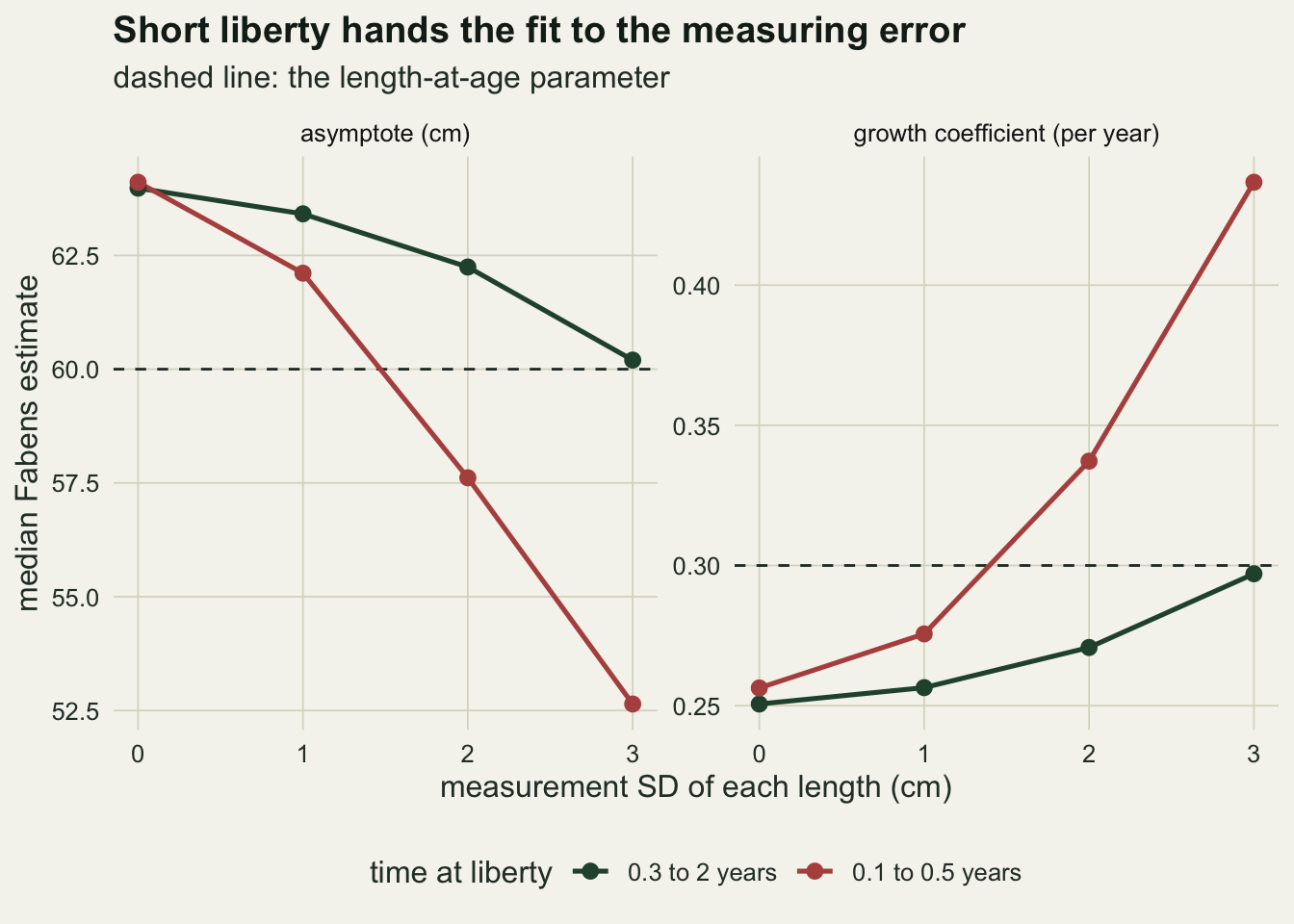
Modelling the fish instead of the increment
The repair developed in the literature does not fit the increments at all. Wang, Thomas and Somers 1995 made the asymptote random in a likelihood that allows for the unknown age at tagging, and Laslett, Eveson and Polacheck 2002 wrote down the joint density of the release and recapture lengths, with the asymptote and the age at tagging both random. For a given age at tagging, both lengths are linear in the fish’s normal asymptote, so the pair is bivariate normal; the unknown age is integrated out numerically over a distribution with its own parameters. The age distribution fitted here is a lognormal, integrated over 24 quantile nodes, with the measurement error variance estimated as well. The fit has six parameters and gives the among-fish spread of the asymptote as one of them.
The test is whether this model recovers the length-at-age parameters when its release-age distribution is wrong. The three designed distributions are not lognormal; a fourth, lognormal, set is added as the case the model gets right. It is also the shape closest to what selective gear usually delivers, so in this post correct specification and realism coincide, which flatters the joint model.
joint_nll <- function(p, len1, len2, at_lib, m = 24) {
  mu <- exp(p[1]); s_l <- exp(p[2]); k <- exp(p[3]); s_m <- exp(p[6])
  a_node <- qlnorm((seq_len(m) - 0.5) / m, p[4], exp(p[5]))
  g1 <- rep(1 - exp(-k * a_node), each = length(len1))
  g2 <- 1 - exp(-k * outer(at_lib, a_node, "+"))
  s11 <- s_l^2 * g1^2 + s_m^2; s22 <- s_l^2 * g2^2 + s_m^2; s12 <- s_l^2 * g1 * g2
  det_s <- s_m^2 * (s_l^2 * (g1^2 + g2^2) + s_m^2)
  z1 <- len1 - mu * g1; z2 <- len2 - mu * g2
  quad <- (s22 * z1^2 - 2 * s12 * z1 * z2 + s11 * z2^2) / det_s
  dens <- exp(-0.5 * quad) / sqrt(det_s)
  val <- length(len1) * log(2 * pi) - sum(log(rowMeans(dens) + 1e-300))
  if (is.finite(val)) val else 1e10
}
fit_joint <- function(d) {
  fb <- fit_fabens(d$len1, d$len2, d$at_lib)
  age_guess <- -log(pmax(1 - pmax(d$len1, 1) / (fb[["linf"]] + 5), 0.02)) / fb[["k"]]
  lo <- c(log(20), log(0.1), log(0.02), -3, log(0.05), log(0.05))
  hi <- c(log(200), log(40), log(2), 4, log(2), log(10))
  p0 <- c(log(fb[["linf"]]), log(3), log(fb[["k"]]), mean(log(age_guess)),
          log(sd(log(age_guess))), log(1))
  p0 <- pmin(pmax(p0, lo + 1e-3), hi - 1e-3)
  o <- nlminb(p0, joint_nll, len1 = d$len1, len2 = d$len2, at_lib = d$at_lib,
              lower = lo, upper = hi)
  n_try <- 0
  while (o$convergence != 0 && n_try < 3) {   # restart from where it stopped
    o <- nlminb(o$par, joint_nll, len1 = d$len1, len2 = d$len2, at_lib = d$at_lib,
                lower = lo, upper = hi)
    n_try <- n_try + 1
  }
  c(linf = exp(o$par[1]), sd_linf = exp(o$par[2]), k = exp(o$par[3]),
    sd_meas = exp(o$par[6]), code = o$convergence,
    fb_linf = fb[["linf"]], fb_k = fb[["k"]])
}
n_rep_joint <- 100   # the joint fit is several hundred times slower
shape_all <- c(age_lev, "lognormal")
set.seed(7315)
joint_raw <- lapply(shape_all, function(sh) t(replicate(n_rep_joint, {
  d <- tag_fish(n_fish, 6, 2, sh)
  c(fit_joint(d), setNames(fit_age_length(d$age1, d$len1), c("al_linf", "al_k")))
})))
names(joint_raw) <- shape_all
jq <- function(sh, col, fun = median) fun(joint_raw[[sh]][, col])
n_code <- sum(vapply(joint_raw, function(x) sum(x[, "code"] != 0), 0))
mcse_joint <- max(vapply(joint_raw, function(x) 1.2533 * sd(x[, "linf"]) / sqrt(n_rep_joint), 0))
sd_ratio <- range(vapply(shape_all, function(sh) jq(sh, "linf", sd) / jq(sh, "fb_linf", sd), 0))
sd_ratio_k <- range(vapply(shape_all, function(sh) jq(sh, "k", sd) / jq(sh, "fb_k", sd), 0))
closer_both <- vapply(shape_all, function(sh)
  abs(jq(sh, "linf") - mu_set) < abs(jq(sh, "fb_linf") - mu_set) &
    abs(jq(sh, "k") - K_set) < abs(jq(sh, "fb_k") - K_set), logical(1))
jd <- function(sh, col, truth) sprintf(if (truth > 1) "%.1f" else "%.3f", abs(jq(sh, col) - truth))
n_joint_total <- n_rep_joint * length(shape_all)
meth_lev <- c("Fabens", "joint likelihood", "length at known age")
jl <- do.call(rbind, lapply(shape_all, function(sh) {
x <- joint_raw[[sh]]
cols <- list(c("fb_linf", "fb_k"), c("linf", "k"), c("al_linf", "al_k"))
do.call(rbind, lapply(1:3, function(i) {
ci <- match(cols[[i]], colnames(x))
rbind(data.frame(shape = sh, method = meth_lev[i], par = "asymptote (cm)",
med = median(x[, ci[1]]), lo = quantile(x[, ci[1]], 0.1),
hi = quantile(x[, ci[1]], 0.9), truth = mu_set),
data.frame(shape = sh, method = meth_lev[i], par = "growth coefficient (per year)",
med = median(x[, ci[2]]), lo = quantile(x[, ci[2]], 0.1),
hi = quantile(x[, ci[2]], 0.9), truth = K_set))
}))
}))
jl$shape <- factor(jl$shape, levels = shape_all)
jl$method <- factor(jl$method, levels = meth_lev)
ggplot(jl, aes(shape, med, colour = method)) +
geom_hline(aes(yintercept = truth), colour = te_body, linetype = "dashed", linewidth = 0.5) +
geom_errorbar(aes(ymin = lo, ymax = hi), width = 0.25, linewidth = 0.6,
position = position_dodge(width = 0.6)) +
geom_point(size = 2.4, position = position_dodge(width = 0.6)) +
facet_wrap(~ par, scales = "free_y", ncol = 1) +
scale_colour_manual(values = c(te_rust, te_forest, te_gold), name = NULL) +
labs(x = "release-age distribution", y = "estimate",
title = "The joint model leans on its age distribution",
subtitle = "dashed line: the length-at-age parameter") +
theme_datasheet() + theme(legend.position = "bottom")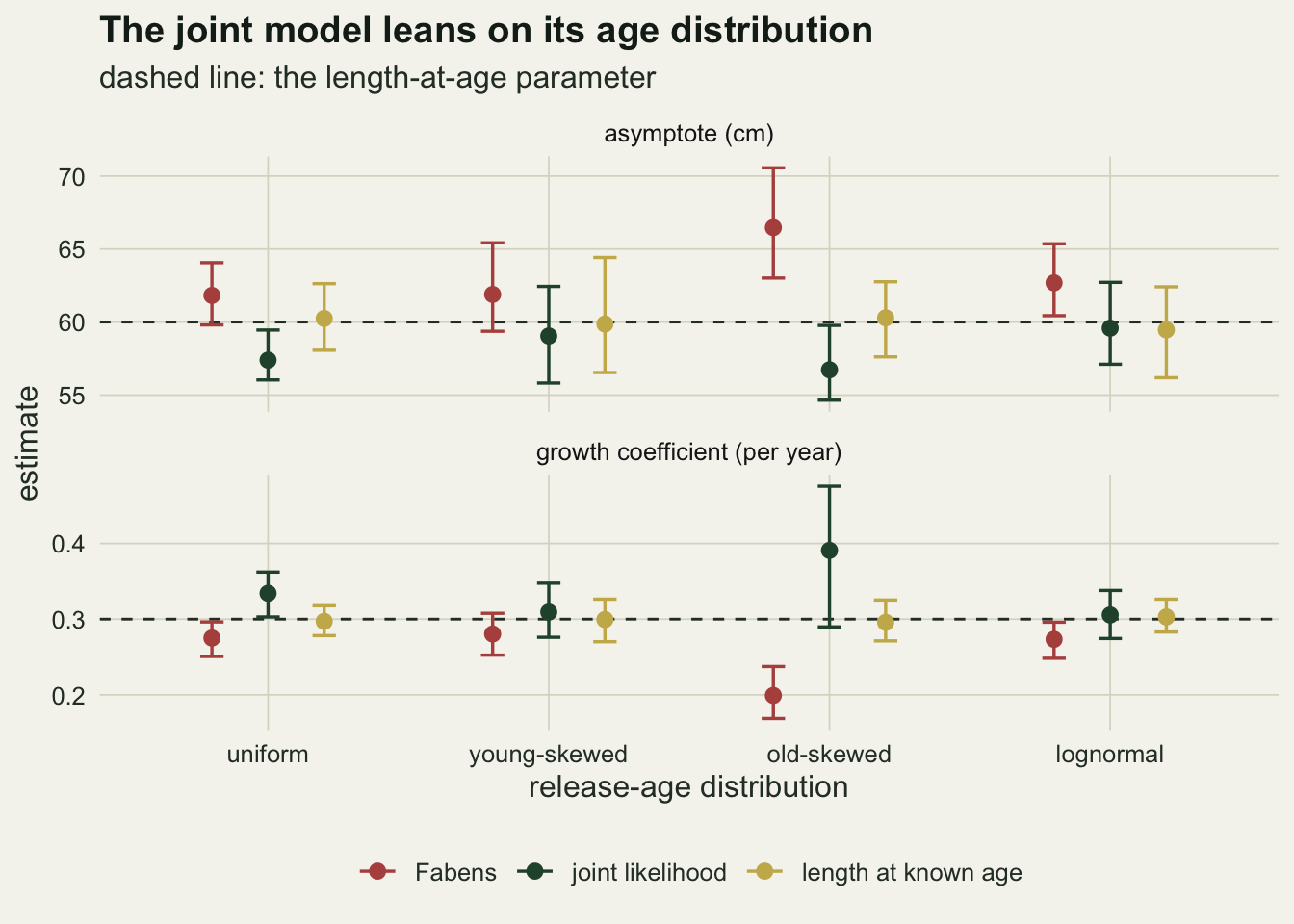
With lognormal release ages, the case the joint model is written for, its median asymptote is 59.6 cm and its median growth coefficient 0.306, against 62.7 cm and 0.273 from the Fabens fit to the same data sets and 59.5 cm and 0.303 from length at the true ages. It also estimates what the Fabens fit cannot: a median among-fish spread of 6.2 cm and a median measurement error of 1.97 cm, against true values of 6 and 2. The largest Monte Carlo standard error of a median joint asymptote in the four sets is 0.35 cm.
When the release ages are not lognormal the joint model misses too, and in the opposite direction to the Fabens fit. For uniform ages its medians are 57.4 cm and 0.334, where the Fabens fit gave 61.8 cm and 0.275. For old-skewed ages they are 56.7 cm and 0.391, where the Fabens fit gave 66.5 cm and 0.199. For young-skewed ages they are 59.0 cm and 0.309, against 61.9 cm and 0.280. Measured as distance from the length-at-age values, the joint model is further off than the Fabens fit on both parameters for uniform ages (asymptote 2.6 against 1.8 cm, growth coefficient 0.034 against 0.025). For young-skewed ages it is closer on both (1.0 against 1.9 cm, 0.009 against 0.020), and for old-skewed ages it is closer on both as well, by a wide margin on the asymptote (3.3 against 6.5 cm) but only slightly on the growth coefficient (0.091 against 0.101), where its central eighty per cent range is much wider. Counting the lognormal set, the joint model is closer on both parameters in 3 of the 4 sets. The spread estimates stay near the true 6 cm in every set (medians from 5.6 to 6.2 cm); what goes wrong is the mean curve, because the age distribution decides how the release lengths map onto ages. The replicate standard deviation of the joint asymptote is between 0.81 and 1.21 times that of the Fabens asymptote across the four sets, and for the growth coefficient the ratio is between 1.18 and 3.09. After up to three restarts, 0 of the 400 joint fits still ended with a non-zero convergence code; they are kept in the summaries.
The joint likelihood matches how tagged fish actually come to have the lengths they have, and it is the only one of the two fits that says anything about individual variation. Under the lognormal set, the shape closest to what selective gear usually delivers and also the one it assumes, it recovered the length-at-age values; under 2 of the 3 misspecified shapes it was still closer than the Fabens fit on both parameters, and under uniform ages it did worse. It is not a free correction. It turns a question about increments into a question about the age structure of the tagged fish, and a wrong answer to that question moves the growth curve.
What to report
Say which data the growth parameters came from, in the same sentence as the parameters. An asymptote and growth coefficient from a Fabens fit to increments are not the parameters of the mean length-at-age curve, and Francis 1988 made exactly this point: the two kinds of data give parameters with different meanings. Plugging tagging estimates into a model built on length at age, or comparing them with an age-length study of another population, compares two different things.
Report the time-at-liberty distribution and how the release and recapture lengths were measured, with an estimate of measurement error if the programme has one (repeat measurements of the same fish on one day are enough). The figures above show that the error decides whether the Fabens fit lands above or below the length-at-age values, and that short times at liberty make it worse. Fish recaptured within a few weeks carry more measuring noise than growth and can be excluded, and the cut-off should be stated.
Report the size or age structure of the tagged fish, not just the recaptures. It sets the size of the asymptote-spread bias for the Fabens fit and the size of the misspecification bias for a joint likelihood, so a reader cannot judge either without it.
If a joint likelihood is fitted, report the release-age distribution that was assumed, the fitted spread of the asymptote and the fitted measurement error, and refit with at least one other age distribution. If the mean curve moves when the age model changes, that movement is part of the uncertainty.
If what is wanted is how fast fish of the sizes that were tagged actually grow, the increments answer that directly. Francis 1988 proposed alternative parameterisations of the tagging model for this reason, such as mean annual growth at two reference lengths inside the tagged range, which describe what the increments measure and do not pretend to be a length-at-age curve.
Honest limits
Every fish here follows a von Bertalanffy curve exactly, with zero length at age zero, an asymptote that is normal and independent of age at tagging, and measurement errors that are normal, independent and equal at release and recapture. Real growth is seasonal, so an increment depends on which part of the year a fish was at liberty; tagging and handling often slow growth for a while; and release and recapture lengths are commonly taken by different people with different error. None of these was simulated, and each adds a bias of its own to the Fabens fit.
Age at tagging and the asymptote were drawn independently, and every tagged fish was recaptured. In a real programme recapture depends on size and survival, fast-growing fish may be caught sooner or reach the fishery’s size limit earlier, and the recaptured fish are not a random sample of the tagged ones. That selection works on exactly the covariance between asymptote and release length that drives the Fabens bias, so it can make the bias larger or smaller than shown.
Individual variation in the growth coefficient was added in one small arm only, independently of the asymptote. Among real fish the two are often negatively correlated, and Sainsbury 1980 argues that the joint distribution of the two parameters has to be considered; the direction measured here for independent variation should not be read as the answer for correlated variation.
The joint likelihood was tested in one cell, a 6 cm asymptote spread and 2 cm error, with 100 data sets per release-age distribution and no interval estimates, so nothing is said about its coverage. Its age distribution was a single lognormal. More flexible choices, such as mixtures or an age distribution informed by a length-frequency sample of the tagged population, may remove much of the misspecification bias measured here; none was tried. The Wang, Thomas and Somers 1995 likelihood was not coded; the one here follows the joint-density formulation of Laslett and colleagues.
The Fabens fit was unweighted least squares with Gauss-Newton standard errors. Maximum likelihood versions with a variance model for the increments, as used in practice for tagging data, change the weights given to small and large fish. They were not run, and the sizes of both biases measured here should not be carried over to them.
References
Sainsbury KJ 1980 Canadian Journal of Fisheries and Aquatic Sciences 37(2):241-247 (10.1139/f80-031)
Francis RICC 1988 Canadian Journal of Fisheries and Aquatic Sciences 45(6):936-942 (10.1139/f88-115)
Wang YG, Thomas MR, Somers IF 1995 Canadian Journal of Fisheries and Aquatic Sciences 52(2):252-259 (10.1139/f95-025)
Laslett GM, Eveson JP, Polacheck T 2002 Canadian Journal of Fisheries and Aquatic Sciences 59(6):976-986 (10.1139/f02-069)