library(ggplot2)
library(patchwork)
library(nlme)

te_paper  <- "#f5f4ee"
te_ink    <- "#16241d"
te_body   <- "#2c3a31"
te_forest <- "#275139"
te_rust   <- "#b5534e"
te_gold   <- "#c9b458"
te_line   <- "#dad9ca"

theme_datasheet <- function() {
  theme_minimal(base_size = 12) +
    theme(plot.background  = element_rect(fill = te_paper, colour = NA),
          panel.background = element_rect(fill = te_paper, colour = NA),
          panel.grid.major = element_line(colour = te_line, linewidth = 0.3),
          panel.grid.minor = element_blank(),
          text             = element_text(colour = te_body),
          plot.title       = element_text(colour = te_ink, face = "bold"),
          plot.subtitle    = element_text(colour = te_body),
          axis.text        = element_text(colour = te_body))
}Individual growth curves with nlme
R
nlme
mixed models
nonlinear regression
growth
simulation
ecology tutorial
Averaging per-fish nls fits overstates how much fish differ in asymptotic length when ages stop short. Individual von Bertalanffy growth curves in R with nlme.
A reservoir population of pike has been tagged for twelve years. Fish are marked as juveniles of known age and measured again whenever they turn up in a fyke net, so every animal has its own short run of length at age: three or four measurements for most fish, six or more for a few. The biology is about individuals. How large do fish in this water grow, and how much do they differ in the size they level off at? That second number, the among-individual spread of the asymptote, is what a model of size-dependent fecundity or of harvest slot limits needs.
The tempting route is two stages. Fit a von Bertalanffy curve to each fish with nls, collect the sixty asymptotes, and report their mean and standard deviation. The alternative is a nonlinear mixed model: one fit in nlme in which each fish’s asymptote and growth coefficient are random draws around population values, so the spread among fish is estimated as a parameter rather than read off a column of estimates.
The same argument on a linear predictor is already on the site. The post on community covariates and species traits fits each species’ occupancy slope on its own (on the logit scale), drops any species without a finite estimate, and shows the spread of the independent slopes falling once the slopes are pooled in a hierarchical Bayesian occupancy model. The post on random slopes in mixed models shows the same partial pooling for twelve linear regressions. In neither does a parameter enter the mean curve nonlinearly the way an asymptote does, and the growth curve adds something that no linear shrinkage argument predicts: a fish whose oldest measurement is still on the steep part of the curve returns an asymptote that is not merely noisy but skewed, with a long upper tail. The post on fitting growth curves with nls shows exactly this for one pooled sample of young fish (the asymptote becomes an extrapolation with a lopsided profile interval); here that happens fish by fish, and the question is what it does to a population summary built from the fish-level fits.
Sixty fish and three measurements each
The generating model gives fish i an asymptote drawn from a normal distribution with mean 60 cm and standard deviation 6 cm, and a growth coefficient whose logarithm is normal around log 0.3 with standard deviation 0.2. The two are drawn independently. Each fish is measured at a set of distinct ages sampled without replacement from ages one to twelve, and each length carries independent measurement error with standard deviation 3 cm. The curve is written without the t0 term, so it passes through zero length at age zero, and both analyses below use the same two-parameter form. All of these constants were fixed before any fit was run.
n_fish  <- 60            # tagged fish per data set
linf_mu <- 60            # population mean asymptote, cm
linf_sd <- 6             # among-fish SD of the asymptote, cm
k_mu    <- 0.3           # median growth coefficient, per year
logk_sd <- 0.2           # among-fish SD of log k
meas_sd <- 3             # measurement error SD, cm
age_max <- 12            # ages sampled from 1 to age_max

vb <- function(age, Linf, k) Linf * (1 - exp(-k * age))

sim_fish <- function(n_age, amax = age_max) {
  linf_i <- rnorm(n_fish, linf_mu, linf_sd)
  k_i    <- exp(rnorm(n_fish, log(k_mu), logk_sd))
  ages   <- unlist(lapply(seq_len(n_fish), function(i) sort(sample.int(amax, n_age))))
  id     <- rep(seq_len(n_fish), each = n_age)
  list(dat = data.frame(fish = factor(id), age = ages,
                        len = vb(ages, linf_i[id], k_i[id]) + rnorm(n_fish * n_age, 0, meas_sd)),
       linf_i = linf_i, k_i = k_i)
}
Both analyses need starting values, and they get the same ones: the estimates from a single nls curve fitted to all fish pooled, which is what an analyst would do first anyway. (That pooled fit is itself started from the largest observed length and k = 0.3, which happens to be the generating median; the per-fish and mixed-model fits never see this guess, only the pooled estimates it converges to.) A per-fish fit that fails from that start is tried again from three deliberately different starts before it is counted as a failure, so the two-stage route is given more help than the mixed model, which gets one start and no retry. The mixed model has random asymptote and random growth coefficient with an unstructured two by two covariance (pdSymm), independent residuals with constant variance, and default nlme controls. Warnings raised inside its iterations are counted rather than printed. nlme alternates a penalised nonlinear least squares step for the fish-level parameters with a linear mixed-model step for the fixed effects and variance components, the algorithm of Lindstrom and Bates 1990, and Pinheiro and Bates 2000 is the reference for the model syntax and the pdSymm covariance class.
alt_starts <- list(c(Linf = 80, k = 0.15), c(Linf = 50, k = 0.5), c(Linf = 120, k = 0.08))

fit_nls_fish <- function(di, start) {
  try_fit <- function(s) tryCatch(nls(len ~ vb(age, Linf, k), data = di, start = as.list(s)),
                                  error = function(e) NULL)
  f <- try_fit(start); first_ok <- !is.null(f)
  if (!first_ok) for (s in alt_starts) { f <- try_fit(s); if (!is.null(f)) break }
  if (is.null(f)) return(c(Linf = NA, k = NA, se_Linf = NA, first_ok = 0))
  cf <- summary(f)$coefficients
  c(Linf = cf["Linf", 1], k = cf["k", 1], se_Linf = cf["Linf", 2], first_ok = as.numeric(first_ok))
}

fit_both <- function(dat) {
  pool <- coef(nls(len ~ vb(age, Linf, k), data = dat, start = list(Linf = max(dat$len), k = 0.3)))
  est  <- t(vapply(split(dat, dat$fish), fit_nls_fish, numeric(4), start = pool))
  n_warn <- 0
  mm <- withCallingHandlers(
    tryCatch(nlme(len ~ vb(age, Linf, k), data = dat, groups = ~ fish,
                  fixed = Linf + k ~ 1, random = pdSymm(Linf + k ~ 1), start = pool),
             error = function(e) NULL),
    warning = function(w) { n_warn <<- n_warn + 1; invokeRestart("muffleWarning") })
  list(est = est, mm = mm, n_warn = n_warn, pool = pool)
}set.seed(4417)
ex_sim <- sim_fish(3)
ex <- fit_both(ex_sim$dat)
ex_ok <- !is.na(ex$est[, "Linf"])
ex_nls <- ex$est[ex_ok, "Linf"]
ex_coef <- coef(ex$mm)
ex_blup <- setNames(ex_coef$Linf, rownames(ex_coef))
ex_blup_k <- setNames(ex_coef$k, rownames(ex_coef))
ex_nl_sd <- as.numeric(VarCorr(ex$mm)["Linf", "StdDev"])
ex_fail <- sum(!ex_ok); ex_first_fail <- sum(ex$est[, "first_ok"] == 0)
ex_max <- max(ex_nls); ex_min <- min(ex_nls)
ex_n_over <- sum(ex_nls > linf_mu + 3 * linf_sd)In one simulated data set with three measurements per fish, 58 of the 60 per-fish fits return estimates (2 failed from the pooled start and 2 still failed after the retries). The asymptotes from those fits have mean 62.2 cm and standard deviation 9.7 cm, and they run from 42.5 to 89.6 cm; 4 of them lie more than three true standard deviations above the true mean. The realised asymptotes of the sixty simulated fish have mean 60.0 and standard deviation 7.0. The mixed model on the same data returns a population mean asymptote of 62.0 cm and an among-fish standard deviation of 5.0 cm, with 0 warnings raised inside its iterations. One data set is noisy for both routes, and here the mixed model’s mean is also high; the grid below shows which way each route errs on average.
pick <- names(sort(ex_nls, decreasing = TRUE))[1:3]
pick <- c(pick, names(sort(abs(ex_nls - median(ex_nls))))[1:3])
age_grid <- seq(0, age_max, length.out = 100)
curve_rows <- do.call(rbind, lapply(pick, function(f) {
  rbind(data.frame(fish = f, age = age_grid, len = vb(age_grid, ex$est[f, "Linf"], ex$est[f, "k"]),
                   fit = "per-fish nls"),
        data.frame(fish = f, age = age_grid, len = vb(age_grid, ex_blup[f], ex_blup_k[f]),
                   fit = "nlme, fish-level"),
        data.frame(fish = f, age = age_grid,
                   len = vb(age_grid, ex_sim$linf_i[as.integer(f)], ex_sim$k_i[as.integer(f)]),
                   fit = "true curve"))
}))
curve_rows$fit <- factor(curve_rows$fit, levels = c("true curve", "per-fish nls", "nlme, fish-level"))
curve_rows$fish <- factor(paste("fish", curve_rows$fish), levels = paste("fish", pick))
pts <- ex_sim$dat[ex_sim$dat$fish %in% pick, ]
pts$fish <- factor(paste("fish", pts$fish), levels = paste("fish", pick))
ggplot(curve_rows, aes(age, len)) +
  geom_line(aes(colour = fit, linetype = fit), linewidth = 0.8) +
  geom_point(data = pts, colour = te_ink, size = 2) +
  facet_wrap(~ fish, nrow = 2) +
  scale_x_continuous(breaks = c(0, 4, 8, 12)) +
  scale_colour_manual(values = c(te_gold, te_rust, te_forest), name = NULL) +
  scale_linetype_manual(values = c("dashed", "solid", "solid"), name = NULL) +
  coord_cartesian(ylim = c(0, 110)) +
  labs(x = "age (years)", y = "length (cm)",
       title = "Three points do not fix an asymptote",
       subtitle = "top row: the three largest nls asymptotes; bottom row: three near the median") +
  theme_datasheet() + theme(legend.position = "bottom")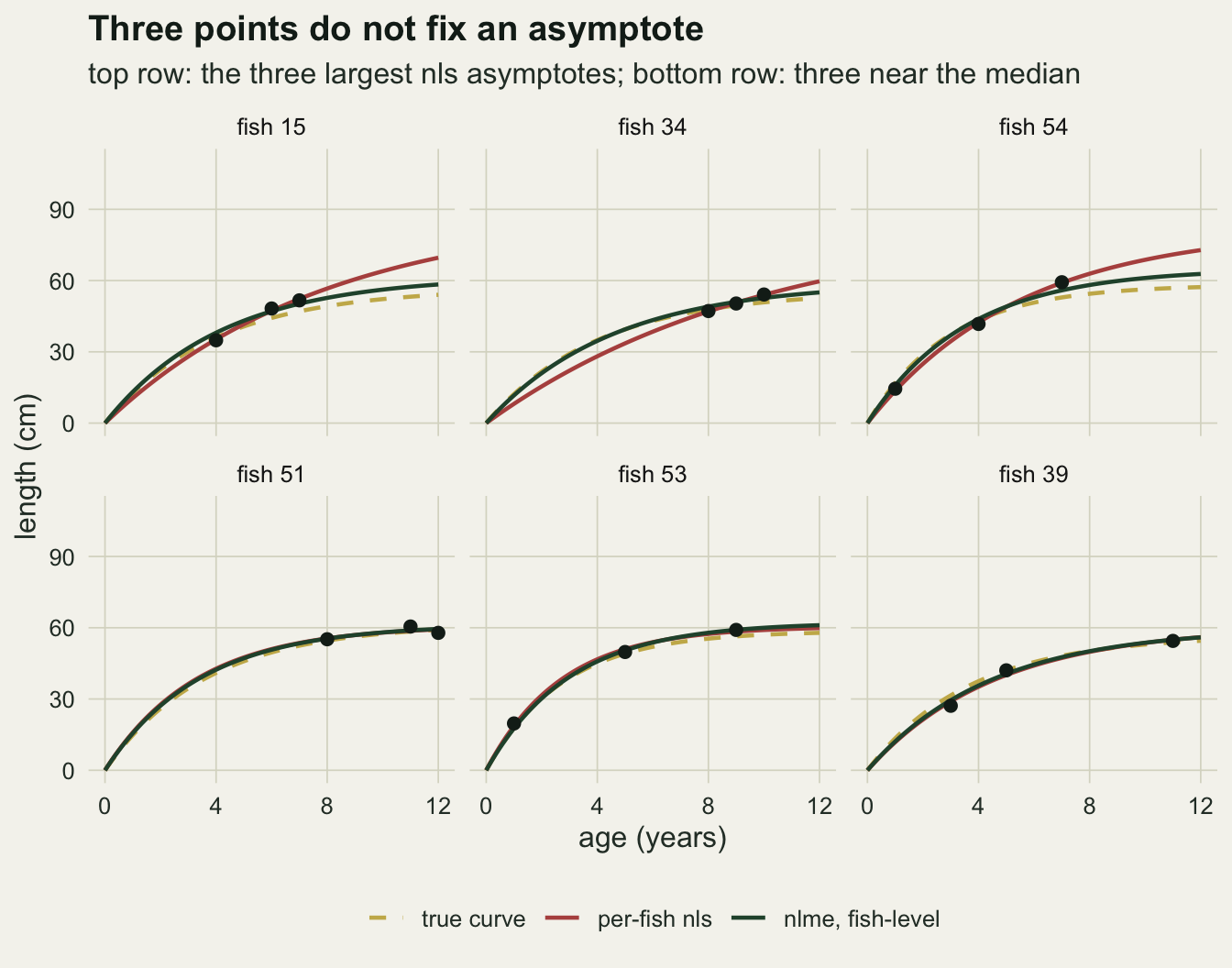
The top row is the problem in miniature. Three points with a little measurement error can be joined by a curve that is still climbing at age twelve: a slower growth coefficient and a higher asymptote fit them nearly as well as the truth, and least squares takes whichever combination the noise happens to favour. The rust curves in the top row keep rising where the true curves have flattened. The mixed model’s fish-level curves for the same fish sit much closer to the truth, because the population says asymptotes that large are rare. In the bottom row the points include ages near or past the plateau, and all three fits nearly coincide.
Where the wild asymptotes come from
If the upper tail is an extrapolation artefact, the error in a fish’s asymptote should depend on how close to its plateau that fish was at its last measurement. The true fraction of the asymptote reached at the oldest sampled age, one minus exp(-k times that age), measures it. Ten data sets of the same design give six hundred fish to look at.
set.seed(7302)
mech <- do.call(rbind, lapply(seq_len(10), function(r) {
  s  <- sim_fish(3)
  fb <- fit_both(s$dat)
  oldest <- tapply(s$dat$age, s$dat$fish, max)
  data.frame(frac = 1 - exp(-s$k_i * oldest),
             err_nls = fb$est[, "Linf"] - s$linf_i,
             err_nlme = if (is.null(fb$mm)) NA else
               coef(fb$mm)[levels(s$dat$fish), "Linf"] - s$linf_i)
}))
mech_ok <- !is.na(mech$err_nls)
low_frac <- mech$frac < 0.85
q_nls_low  <- quantile(mech$err_nls[mech_ok & low_frac], c(0.1, 0.5, 0.9))
q_nls_high <- quantile(mech$err_nls[mech_ok & !low_frac], c(0.1, 0.5, 0.9))
q_nlme_low <- quantile(mech$err_nlme[low_frac], c(0.1, 0.5, 0.9), na.rm = TRUE)
share_low  <- mean(low_frac)
fail_low   <- mean(!mech_ok[low_frac]); fail_high <- mean(!mech_ok[!low_frac])
n_clip     <- sum(mech$err_nls[mech_ok] > 60 | mech$err_nls[mech_ok] < -30) +
              sum(mech$err_nlme > 60 | mech$err_nlme < -30, na.rm = TRUE)
tail_ratio <- q_nls_low[[3]] / abs(q_nls_low[[1]])
big_up <- mech_ok & mech$err_nls > 2 * linf_sd
share_big_low <- mean(low_frac[big_up]); n_big_up <- sum(big_up)
n_mech_err <- sum(is.na(mech$err_nlme)) / n_fish
mean_err_nls <- mean(mech$err_nls[mech_ok]); med_err_nls <- median(mech$err_nls[mech_ok])
Of the 600 fish, 9.8 per cent had reached less than 85 per cent of their own asymptote by their oldest measurement. For those fish the per-fish nls error in the asymptote has a median of +2.8 cm, but its 10th and 90th percentiles are -12.5 and +26.4 cm, so the 90th percentile lies 2.1 times as far above zero as the 10th lies below it. For the fish that had reached 85 per cent or more the same percentiles are -5.2, +0.4 and +7.8 cm. The short-of-plateau fish are a minority, yet they supply 39 per cent of the 44 asymptotes that overshoot the truth by more than two true standard deviations. That lopsided tail is why the mean error of the per-fish asymptotes over all fish is +1.83 cm while the median error is +0.54 cm.
The mixed model’s fish-level asymptotes for the same short-of-plateau fish have 10th, 50th and 90th error percentiles of -3.6, -0.3 and +6.7 cm. They have smaller errors, but because they are shrunk towards the population mean: a fish that really is large is pulled down, which matters when ranking individuals (more on that under What to report). nlme stopped with an error in 0 of these ten data sets. In the figure, 2 errors fall outside the plotted range and are not drawn.
mech_long <- rbind(data.frame(frac = mech$frac, err = mech$err_nls, fit = "per-fish nls"),
                   data.frame(frac = mech$frac, err = mech$err_nlme, fit = "nlme, fish-level"))
mech_long$fit <- factor(mech_long$fit, levels = c("per-fish nls", "nlme, fish-level"))
mech_long <- mech_long[!is.na(mech_long$err), ]
ggplot(mech_long, aes(frac, err, colour = fit)) +
  geom_hline(yintercept = 0, colour = te_body, linetype = "dashed", linewidth = 0.5) +
  geom_vline(xintercept = 0.85, colour = te_line, linewidth = 0.8) +
  geom_point(alpha = 0.45, size = 1.3) +
  facet_wrap(~ fit) +
  scale_colour_manual(values = c(te_rust, te_forest), guide = "none") +
  coord_cartesian(ylim = c(-30, 60)) +
  labs(x = "fraction of the true asymptote reached at the oldest measured age",
       y = "estimated minus true asymptote (cm)",
       title = "The long tail grows where the plateau was never seen",
       subtitle = "600 fish, three measurements each; vertical axis clipped at -30 and 60 cm") +
  theme_datasheet()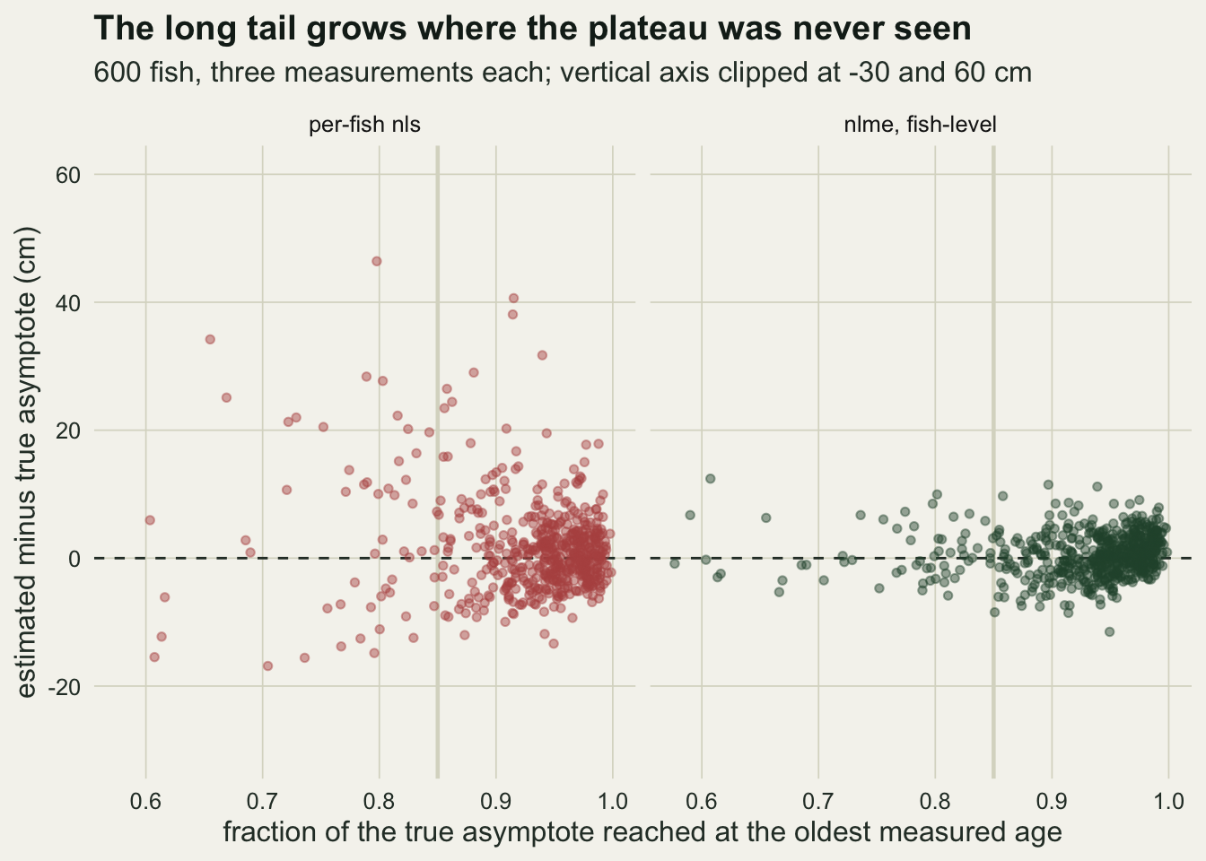
Over replicates and sampling densities
One data set proves nothing about a procedure. The grid below repeats both analyses at three, four, six and ten measurements per fish with ages drawn from one to twelve, plus one extra cell with four measurements drawn from ages one to eight, which keeps the number of points per fish and takes away the old ages. The number of replicates per cell, 50, was set from a timing pilot so the page builds in a few minutes, before any summary was inspected; it is small, so every comparison below carries its Monte Carlo standard error.
n_rep <- 50
cells <- data.frame(n_age = c(3, 4, 6, 10, 4), amax = c(12, 12, 12, 12, 8))
cells$label <- factor(sprintf("%d ages from 1-%d", cells$n_age, cells$amax),
                      levels = sprintf("%d ages from 1-%d", cells$n_age, cells$amax))

one_rep <- function(n_age, amax) {
  s  <- sim_fish(n_age, amax)
  fb <- fit_both(s$dat)
  ok <- !is.na(fb$est[, "Linf"]); L <- fb$est[ok, "Linf"]; se_L <- fb$est[ok, "se_Linf"]
  mm <- fb$mm
  nl_ci <- if (is.null(mm)) c(NA, NA, NA) else
    tryCatch(intervals(mm, which = "fixed")$fixed["Linf", ], error = function(e) c(NA, NA, NA))
  c(fail_first = sum(fb$est[, "first_ok"] == 0), fail = sum(!ok),
    ts_mean = mean(L), ts_median = median(L), ts_sd = sd(L),
    ts_corr_sd = sqrt(max(0, var(L) - mean(se_L^2))), ts_corr_neg = var(L) - mean(se_L^2) < 0,
    ts_cover = unname(abs(mean(L) - linf_mu) <= qt(0.975, sum(ok) - 1) * sd(L) / sqrt(sum(ok))),
    nl_error = is.null(mm), nl_warn = fb$n_warn,
    nl_mean = if (is.null(mm)) NA else unname(fixef(mm)["Linf"]),
    nl_sd = if (is.null(mm)) NA else as.numeric(VarCorr(mm)["Linf", "StdDev"]),
    nl_cover = unname(nl_ci[1] <= linf_mu & linf_mu <= nl_ci[3]))
}

set.seed(9051)
t_start <- proc.time()[["elapsed"]]
grid_raw <- lapply(seq_len(nrow(cells)), function(j)
  t(replicate(n_rep, one_rep(cells$n_age[j], cells$amax[j]))))
grid_secs <- proc.time()[["elapsed"]] - t_start

summ <- do.call(rbind, lapply(seq_len(nrow(cells)), function(j) {
  g <- grid_raw[[j]]
  m_se <- function(v) c(mean(v, na.rm = TRUE), sd(v, na.rm = TRUE) / sqrt(sum(!is.na(v))))
  rbind(
    data.frame(label = cells$label[j], method = "two-stage", what = "mean",
               est = m_se(g[, "ts_mean"])[1], mcse = m_se(g[, "ts_mean"])[2]),
    data.frame(label = cells$label[j], method = "two-stage median", what = "mean",
               est = m_se(g[, "ts_median"])[1], mcse = m_se(g[, "ts_median"])[2]),
    data.frame(label = cells$label[j], method = "nlme", what = "mean",
               est = m_se(g[, "nl_mean"])[1], mcse = m_se(g[, "nl_mean"])[2]),
    data.frame(label = cells$label[j], method = "two-stage", what = "sd",
               est = m_se(g[, "ts_sd"])[1], mcse = m_se(g[, "ts_sd"])[2]),
    data.frame(label = cells$label[j], method = "two-stage, SE-corrected", what = "sd",
               est = m_se(g[, "ts_corr_sd"])[1], mcse = m_se(g[, "ts_corr_sd"])[2]),
    data.frame(label = cells$label[j], method = "nlme", what = "sd",
               est = m_se(g[, "nl_sd"])[1], mcse = m_se(g[, "nl_sd"])[2]))
}))
gv <- function(lab, meth, wh, col = "est") summ[[col]][summ$label == levels(cells$label)[lab] &
                                                   summ$method == meth & summ$what == wh]
cnt <- t(vapply(grid_raw, function(g) c(
  fail_share = sum(g[, "fail"]) / (n_rep * n_fish),
  first_share = sum(g[, "fail_first"]) / (n_rep * n_fish),
  nl_error = sum(g[, "nl_error"]), nl_warn_reps = sum(g[, "nl_warn"] > 0),
  ts_cover = mean(g[, "ts_cover"]), nl_cover = mean(g[, "nl_cover"], na.rm = TRUE),
  ts_sd_med = median(g[, "ts_sd"]), nl_sd_med = median(g[, "nl_sd"], na.rm = TRUE)), numeric(8)))
n_first_tot <- sum(vapply(grid_raw, function(g) sum(g[, "fail_first"]), 0))
n_rescued <- sum(vapply(grid_raw, function(g) sum(g[, "fail_first"]) - sum(g[, "fail"]), 0))
fail_dense <- sum(cnt[3:4, "fail_share"]); nl_err_other <- sum(cnt[2:4, "nl_error"])
n_neg <- vapply(grid_raw, function(g) sum(g[, "ts_corr_neg"]), 0)
med_corr <- vapply(grid_raw, function(g) median(g[, "ts_corr_sd"]), 0)
n_nl_cov <- vapply(grid_raw, function(g) sum(!is.na(g[, "nl_cover"])), 0)
mcse_cov <- function(p, n) 100 * sqrt(p * (1 - p) / n)
ts_sd_nlok <- vapply(grid_raw, function(g) mean(g[g[, "nl_error"] == 0, "ts_sd"]), 0)
n_nl_ok <- vapply(grid_raw, function(g) sum(g[, "nl_error"] == 0), 0)
The two-stage standard deviation of the asymptote is inflated at every design, and the inflation is set by how far short of the plateau the ages stop. With three ages from one to twelve it averages 11.7 cm over the replicates (Monte Carlo standard error 0.8), 1.94 times the true 6 cm; with four ages 9.6 cm, with six 6.98 cm and with ten 6.53 cm. The cell that keeps four ages but draws them from ages one to eight is larger still, at 14.7 cm (standard error 1.2), worse than three ages from the full range. The number of points per fish is not the driver; whether old fish are in the data is. The replicate distribution of the two-stage SD is itself skewed: its median over replicates is 10.0 cm at three ages and 11.6 cm at four ages from one to eight, below the means, because a few data sets contain one or two absurd asymptotes.
The mixed model’s among-fish SD averages between 5.80 and 6.03 cm across the five cells, with standard errors of at most 0.22. That is within a few tenths of a centimetre of the true value whatever the sampling. Its population mean asymptote ranges from 59.96 to 60.38 cm.
The two-stage mean asymptote is pushed up where the tail is long: 62.11 cm at three ages (standard error 0.23) and 62.45 cm at four ages from one to eight, against 60.17 cm at ten ages. Taking the median of the per-fish asymptotes instead of the mean removes most of that bias (60.84 and 60.47 cm in the two sparse cells), but there is no equally simple repair for the spread.
Correcting the spread does not rescue the two-stage route
The obvious repair is a moment correction: the variance of the per-fish estimates is the among-fish variance plus the average estimation variance, so subtract the mean squared standard error of the per-fish asymptotes before taking the square root. The grid computed it in every replicate, truncating a negative variance at zero, and it is the gold series in the right panel of the figure.
It overcorrects, and by most where the uncorrected value was worst. The moment estimate of the variance was negative, an impossible value set to zero, in 25 of 50 replicates at three ages, 11 at four and 34 at four ages from one to eight (0 and 0 at six and ten ages). Averaged with those zeros, the corrected SD is 2.79 cm at three ages, 4.61 at four and 1.69 cm at four ages from one to eight, with replicate medians of 0.92, 5.39 and 0.00 cm, against a truth of 6. The reason is the same skew. The Wald standard error of a fish that never neared its plateau is enormous, and its square dominates the average; it measures the curvature of a flat likelihood at the point estimate, not the spread of the estimate over repeated sampling. Subtracting it removes far more variance than the extrapolated asymptotes added. At ten ages, where the per-fish fits are near linear in the parameters, the correction gives 5.98 cm and works.
Failed per-fish fits are the usual suspect when a two-stage analysis of sparse data goes wrong, and here there were few. The share of fish whose nls fit failed was 2.8 per cent at three ages, 0.9 per cent at four and 0.2 per cent at four ages from one to eight, and 0.0 per cent at six and ten ages combined. Of the 117 per-fish fits across the whole grid that failed from the pooled start, the three alternative starting values rescued 1, so almost all of these failures belong to the data, not to the start. Dropping a few fish is not what inflates the spread; the fits that do converge are.
The mixed model has its own failures, and they belong in the report. nlme stopped with an error in 2 of 50 replicates at three ages and 3 at four ages from one to eight, and in 0 replicates across the other three cells. Warnings from an inner optimisation step that did not converge appeared in between 2 and 39 replicates per cell, including fits that ended normally; the summaries above use every fit that returned, warned or not. The nlme means and SDs are therefore over the 48 and 47 replicates in which it returned in the two sparse cells; restricted to those replicates the two-stage SD is 11.7 and 14.8 cm, so the comparison does not depend on which replicates nlme dropped. Coverage of the true mean asymptote by the 95 per cent interval from intervals() was 85 per cent at three ages and 87 per cent at four ages from one to eight, against 96 per cent at ten ages; the two-stage t interval on the mean of the per-fish asymptotes covered 76 and 90 per cent in the two sparse cells. With 50 replicates a coverage near 95 per cent has a Monte Carlo standard error of about 3 percentage points, and at the observed values it is larger: 5.1 and 4.9 points for nlme (over the 48 and 47 replicates with an interval), 6.0 and 4.2 for the two-stage interval. These are rough; the nlme intervals in the two sparse cells look short, and the two-stage interval at three ages clearly is.
pd <- position_dodge(width = 0.55)
p_mean <- ggplot(summ[summ$what == "mean", ], aes(label, est, colour = method)) +
  geom_hline(yintercept = linf_mu, colour = te_body, linetype = "dashed", linewidth = 0.5) +
  geom_errorbar(aes(ymin = est - 2 * mcse, ymax = est + 2 * mcse), width = 0.25,
                linewidth = 0.5, position = pd) +
  geom_point(size = 2.3, position = pd) +
  scale_colour_manual(values = c(nlme = te_forest, "two-stage" = te_rust,
                                 "two-stage median" = te_gold), name = NULL) +
  guides(colour = guide_legend(nrow = 2)) +
  labs(x = NULL, y = "estimated mean asymptote (cm)", title = "Population mean",
       subtitle = "dashed line: true mean") +
  theme_datasheet() +
  theme(legend.position = "bottom", axis.text.x = element_text(angle = 30, hjust = 1))
p_sd <- ggplot(summ[summ$what == "sd", ], aes(label, est, colour = method)) +
  geom_hline(yintercept = linf_sd, colour = te_body, linetype = "dashed", linewidth = 0.5) +
  geom_errorbar(aes(ymin = est - 2 * mcse, ymax = est + 2 * mcse), width = 0.25,
                linewidth = 0.5, position = pd) +
  geom_point(size = 2.3, position = pd) +
  scale_colour_manual(values = c(nlme = te_forest, "two-stage" = te_rust,
                                 "two-stage, SE-corrected" = te_gold), name = NULL) +
  labs(x = NULL, y = "estimated among-fish SD (cm)", title = "Among-fish spread",
       subtitle = "dashed line: true SD") +
  guides(colour = guide_legend(nrow = 2)) +
  theme_datasheet() +
  theme(legend.position = "bottom", axis.text.x = element_text(angle = 30, hjust = 1))
p_mean + p_sd + plot_annotation(theme = theme_datasheet())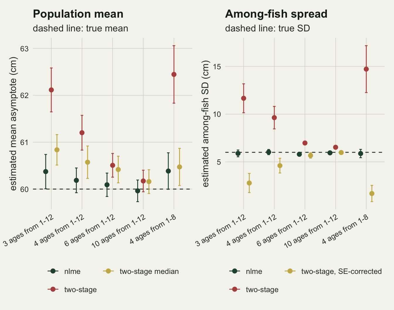
What to report
Report the among-individual standard deviation of the asymptote from a model that estimates it, and say which parameters were random and what covariance was assumed between them. The nlme call above is no longer than a loop over nls, and its variance component is the number a size-structured model downstream actually needs. If a two-stage summary is also shown, say that it is one, and expect it to be larger.
Give the distribution of the oldest measured age per individual, not only the number of measurements. The cell with four ages drawn from one to eight did worse than the cell with three ages from one to twelve, so “four measurements per fish” says little on its own. A histogram of oldest ages, or the share of individuals measured beyond the age at which the population curve reaches most of its asymptote, tells a reader whether any per-individual asymptote was observed or extrapolated.
State how many per-individual fits failed and whether they were dropped, and state how many mixed-model fits raised warnings or errors in any resampling, bootstrap or simulation around the analysis. Both numbers were small here, and neither was what distorted the answer, which is exactly why they should be reported and then set aside rather than treated as the diagnosis.
If a fish-level asymptote is needed for ranking or selecting individuals, do not take it from either route without a warning. The per-fish nls value is an extrapolation with a long upper tail; the mixed-model value is shrunk towards the mean in proportion to how little that fish’s data say. They answer different questions, and neither is a measurement of that fish’s maximum size.
Honest limits
The generating model is the model being fitted. Asymptote and growth coefficient are drawn independently, both are normal on the scales used, the curve has no t0, measurement error is constant and independent, and every fish follows a von Bertalanffy curve exactly. Real growth data break most of these: asymptote and growth coefficient are usually negatively correlated among individuals, lengths at successive ages of one fish carry correlated deviations from any smooth curve, and variance often grows with length. The mixed model recovering the truth here says that it works when it is correctly specified; it says nothing about how it behaves when the random-effects distribution is skewed or the growth form is wrong.
Ages were sampled uniformly without replacement from a fixed window. A tagging study does not work like that. Recapture probability depends on size, fish die, and the oldest measurements come from the survivors, so the individuals that reach old ages in the data are not a random subset. That selection affects both routes and is not measured here.
The per-fish fits used the default Gauss-Newton nls with three fallback starts, and the comparison uses the unweighted mean and standard deviation of their estimates, plus one moment correction. Refined two-stage estimators that iterate between the stages and weight each individual’s estimate by its estimated covariance were not implemented, and they may do better than the simple correction did. The point measured here is narrower: the summaries people actually compute from a column of per-individual estimates.
Fifty replicates per cell is thin. Means and standard deviations carry their Monte Carlo errors in the text and the figure, and the ordering of the cells is clear, but the coverage figures could move by several percentage points with more replication. The sample of sixty fish per data set, the true standard deviation of 6 cm and the measurement error of 3 cm are single choices; a larger measurement error or a smaller among-fish spread should make the two-stage inflation relatively larger and push the mixed model’s variance component towards its own boundary at zero, but neither was run.
Much growth work on tagged animals uses length increments between release and recapture with unknown age (the Fabens form of the von Bertalanffy curve) rather than length at known age. The same mixed-model logic applies there, with the random asymptote entering through the increment equation, but that data type was not simulated.
References
Lindstrom MJ, Bates DM 1990 Biometrics 46(3):673-687 (10.2307/2532087)
Pinheiro JC, Bates DM 2000 Mixed-Effects Models in S and S-PLUS (ISBN 978-0-387-98957-0)