library(ggplot2)
library(patchwork)
library(survival)

te_paper  <- "#f5f4ee"
te_ink    <- "#16241d"
te_body   <- "#2c3a31"
te_forest <- "#275139"
te_rust   <- "#b5534e"
te_gold   <- "#c9b458"
te_line   <- "#dad9ca"

theme_datasheet <- function() {
  theme_minimal(base_size = 12) +
    theme(plot.background  = element_rect(fill = te_paper, colour = NA),
          panel.background = element_rect(fill = te_paper, colour = NA),
          panel.grid.major = element_line(colour = te_line, linewidth = 0.3),
          panel.grid.minor = element_blank(),
          text             = element_text(colour = te_body),
          plot.title       = element_text(colour = te_ink, face = "bold"),
          plot.subtitle    = element_text(colour = te_body),
          axis.text        = element_text(colour = te_body))
}Rock-paper-scissors needs local interaction
R
community ecology
evolutionary game theory
spatial ecology
simulation
survival
ecology tutorial
A well-mixed rock-paper-scissors community soon loses a type; small neighbourhoods on a 40 by 40 lattice keep all three. Censored extinction times in R.
Kerr and colleagues put three strains of Escherichia coli into a game with no winner. A colicin producer kills the sensitive strain, the sensitive strain outgrows the resistant one, and the resistant strain outgrows the producer because it does not pay for the toxin. On a static agar plate, where each colony only meets the colonies beside it, all three strains persisted. In a shaken flask, and on plates whose cells were mixed at every transfer, the sensitive strain was lost and the resistant strain was left alone. The lizard Uta stansburiana has a three-way cycle of male throat morphs that Sinervo and Lively described in the same terms, and intransitive competition among sessile organisms has been proposed often enough that the question is a general one: what does space have to do with keeping a cycle going?
The site has the two halves of the answer in separate posts. The replicator equation in R runs rock-paper-scissors in an infinite, well-mixed population and shows the interior point to be a neutral centre, with frequencies that cycle and never settle. Nothing there is ever lost, because an infinite population cannot drift. Network reciprocity on a lattice is the other half: a prisoner’s dilemma in which cooperator clusters survive on a lattice at benefit-to-cost ratios where a well-mixed population loses them. The mechanism there is clustering, a cooperator surrounded by cooperators collecting benefits from them. The mechanism here is different: there is no cooperation, every type is exploited by one neighbour and exploits another, and what a lattice changes is who can invade whom, and how fast a wave of invasion travels.
The post measures two things in one stochastic model. First, how long a finite well-mixed community keeps all three types, and how that time grows with community size; checking a game theory model shows finite populations drifting around an ESS, and a neutral cycle has no ESS to drift around, so drift has nowhere to stop. Second, what happens to that time when the same invasion rule acts only within a neighbourhood of a given radius on the same lattice. Time to the first loss of a type is a survival time, censored at the end of each run, and it is analysed as one with survival::survfit. The last section asks whether the answer is produced by the update scheme, which is the objection checking a spatial cooperation model raises for lattice games in general.
One invasion rule, one clock
Every site of a square lattice with wrapped edges holds one of three types, numbered 1 to 3, and type 1 beats 2, 2 beats 3, 3 beats 1. The elementary event is the same everywhere in the post. Pick a target site at random and a source site at random from the target’s neighbourhood; if the source’s type beats the target’s, the target takes the source’s type, and otherwise nothing happens. A sweep is as many events as there are sites, so every site is a target once per sweep on average. The mean-field limit of this rule, with the source drawn from the whole population, is the replicator equation for rock-paper-scissors with its conserved product of the three frequencies, so the well-mixed version is the finite, stochastic counterpart of the cycles in the replicator post.
The neighbourhood is either the four orthogonal sites (von Neumann, written radius 0 below), a square of side 2r + 1 around the target for radius r, or the whole lattice. Only the neighbourhood differs between treatments; the event, the rates and the clock are identical.
Doing one event at a time in R is too slow for thousands of sweeps on thousands of sites. The lattice engine below therefore updates many targets at once, but only targets that cannot see each other: the sites are split into classes on a sublattice whose spacing exceeds the radius, so no target’s neighbourhood contains another target of the same class. Updating such a class in one vector operation gives exactly the result of updating its members one after another in any order. Each sweep draws classes at random with replacement, as many draws as there are classes, and each replicate lattice draws its own sequence, so replicates stay independent while being stacked into one state vector that a single operation serves. The spacing is at least eight sites unless a finer one is asked for. Whether batching classes like this is harmless is a separate question from whether a single batch is exact, and the last section shows that it is not always harmless. A sweep counts the product of the three type counts, and the first sweep at which it is zero is the time to first loss.
beaten_by <- function(type) type %% 3 + 1

nbr_offsets <- function(radius) {
  if (radius == 0) return(rbind(c(-1, 0), c(1, 0), c(0, -1), c(0, 1)))
  sq <- expand.grid(dr = -radius:radius, dc = -radius:radius)
  as.matrix(sq[!(sq$dr == 0 & sq$dc == 0), ])
}

run_lattice <- function(side, radius, n_rep, max_sweep, scheme = "batch",
                        trace_every = 0, min_spacing = 8) {
  n_cell <- side * side
  rows <- rep(seq_len(side), times = side)
  cols <- rep(seq_len(side), each = side)
  glob <- is.infinite(radius)
  if (scheme == "sync") {
    cls <- list(seq_len(n_cell))
  } else {
    spacing <- if (glob) side else
      min(Filter(function(d) side %% d == 0 && d > radius && d >= min(min_spacing, side),
                 seq_len(side)))
    cls <- split(seq_len(n_cell), (rows %% spacing) * spacing + cols %% spacing)
  }
  n_cls <- length(cls)
  n_t   <- length(cls[[1]])
  tgt_mat <- matrix(unlist(cls, use.names = FALSE), n_t, n_cls)
  rep_off <- rep((seq_len(n_rep) - 1) * n_cell, each = n_t)
  row_idx <- rep(seq_len(n_t), times = n_rep)
  if (!glob) {
    offs <- nbr_offsets(radius)
    n_nb <- nrow(offs)
    src_arr <- vapply(seq_len(n_nb), function(j)
      ((cols[tgt_mat] + offs[j, 2] - 1) %% side) * side +
        (rows[tgt_mat] + offs[j, 1] - 1) %% side + 1, numeric(n_t * n_cls))
    src_arr <- array(src_arr, c(n_t, n_cls, n_nb))
  }
  n_tr   <- n_t * n_rep
  state  <- sample.int(3, n_cell * n_rep, replace = TRUE)
  bin_off <- rep((seq_len(n_rep) - 1) * 3, each = n_cell)
  loss  <- rep(NA_real_, n_rep)
  trace <- NULL
  for (sw in seq_len(max_sweep)) {
    # each replicate draws its own class schedule
    ord <- if (scheme == "batch") {
      matrix(sample.int(n_cls, n_cls * n_rep, replace = TRUE), n_cls, n_rep)
    } else {
      vapply(seq_len(n_rep), function(j) sample.int(n_cls), numeric(n_cls))
    }
    ord <- matrix(ord, n_cls, n_rep)
    for (step in seq_len(n_cls)) {
      cls_rep <- rep(ord[step, ], each = n_t)
      site <- tgt_mat[row_idx + (cls_rep - 1) * n_t]
      tgt  <- site + rep_off
      if (glob) {
        pick <- sample.int(n_cell - 1, n_tr, replace = TRUE)
        src  <- pick + (pick >= site) + rep_off
      } else {
        nb_pick <- sample.int(n_nb, n_tr, replace = TRUE)
        src <- src_arr[row_idx + (cls_rep - 1) * n_t + (nb_pick - 1) * n_t * n_cls] + rep_off
      }
      s_type <- state[src]
      win <- state[tgt] == beaten_by(s_type)
      state[tgt[win]] <- s_type[win]
    }
    cnt   <- matrix(as.numeric(tabulate(state + bin_off, 3 * n_rep)), n_rep, 3, byrow = TRUE)
    prod3 <- cnt[, 1] * cnt[, 2] * cnt[, 3]
    if (trace_every > 0 && sw %% trace_every == 0)
      trace <- rbind(trace, data.frame(sweep = sw, rep = seq_len(n_rep),
                                       x1 = cnt[, 1] / n_cell,
                                       h = 27 * prod3 / n_cell^3))
    loss[is.na(loss) & prod3 == 0] <- sw
    if (trace_every == 0 && !anyNA(loss)) break
  }
  list(time = ifelse(is.na(loss), max_sweep, loss), lost = !is.na(loss),
       state = state, trace = trace)
}
For the whole-lattice neighbourhood no sublattice separates targets from sources, so the engine above can only do it one site per class, which is exact but slow. The well-mixed control used for timing is instead the same process written on counts. With n1, n2 and n3 sites of each type, an event changes the counts only when the ordered target and source pair is one of the three winning combinations, which has probability (n1 n2 + n2 n3 + n3 n1) over N(N - 1). The waiting time in events to the next effective event is therefore geometric, and which of the three it is follows the three products. That is the exact random-sequential process with a global neighbourhood, one effective event per loop, vectorised across replicates.
run_mixed <- function(n_cell, n_rep, max_sweep) {
  init <- matrix(as.numeric(tabulate(sample.int(3, n_cell * n_rep, TRUE) +
                            rep((seq_len(n_rep) - 1) * 3, each = n_cell), 3 * n_rep)),
                 n_rep, 3, byrow = TRUE)
  n1 <- init[, 1]; n2 <- init[, 2]; n3 <- init[, 3]
  id <- seq_len(n_rep)
  clock <- numeric(n_rep)
  out_time <- rep(max_sweep, n_rep)
  out_lost <- rep(FALSE, n_rep)
  n_pair <- n_cell * (n_cell - 1)
  while (length(id)) {
    r1 <- n1 * n2
    r2 <- n2 * n3
    r_tot <- r1 + r2 + n3 * n1
    clock <- clock + (rgeom(length(id), r_tot / n_pair) + 1) / n_cell
    u  <- runif(length(id)) * r_tot
    e1 <- u <= r1
    e3 <- u > r1 + r2
    e2 <- !e1 & !e3
    n1 <- n1 + e1 - e3
    n2 <- n2 + e2 - e1
    n3 <- n3 + e3 - e2
    done <- (n1 * n2 * n3 == 0) | clock >= max_sweep
    if (any(done)) {
      ext <- done & clock < max_sweep
      out_time[id[ext]] <- clock[ext]
      out_lost[id[ext]] <- TRUE
      keep <- !done
      id <- id[keep]; clock <- clock[keep]
      n1 <- n1[keep]; n2 <- n2[keep]; n3 <- n3[keep]
    }
  }
  list(time = out_time, lost = out_lost)
}
A well-mixed community loses a type
max_sweep <- 2000
n_mixed   <- 40
mixed_n   <- c(400, 900, 1600)

set.seed(4101)
mixed_runs <- lapply(mixed_n, function(n) run_mixed(n, n_mixed, max_sweep))

km_table <- function(run) {
  fit <- survfit(Surv(run$time, run$lost) ~ 1)
  tab <- summary(fit, rmean = max_sweep)$table
  c(median = unname(tab["median"]), lcl = unname(tab["0.95LCL"]),
    ucl = unname(tab["0.95UCL"]), rmean = unname(tab["rmean"]),
    lost = sum(run$lost), n = length(run$lost))
}
mixed_tab <- as.data.frame(t(vapply(mixed_runs, km_table, numeric(6))))
mixed_tab$n_site <- mixed_n
mixed_tab$ratio  <- mixed_tab$median / mixed_n

mixed_slope <- unname(coef(lm(log(median) ~ log(n_site), data = mixed_tab))[2])
n_cens_big  <- sum(!mixed_runs[[3]]$lost)
The design was fixed before any run: 40 replicate communities at each of 400, 900 and 1600 individuals, each started from independent random types and followed to the first loss or to 2000 sweeps.
Every community lost a type before the end of the run except 2 of the 40 at 1600 individuals. Those are right censored: all that is known is that their first loss came after sweep 2000. The Kaplan-Meier estimator uses them correctly, as runs at risk up to the censoring time, where dropping them would bias the median down and setting them to 2000 would bias it down less visibly.
The median time to first loss is 234 sweeps at 400 individuals (95 per cent interval 196 to 296), 437 at 900 (379 to 508) and 718 at 1600 (543 to 1013). Divided by community size those medians are 0.59, 0.49 and 0.45 sweeps per individual. The time grows with N, and the slope of log median on log N is 0.81: a little below strict proportionality over this range, and three sizes with forty runs each are too few to estimate the exponent. Reichenbach, Mobilia and Frey (2006) derived the proportional scaling for large N; what the simulation adds is the constant, about half a sweep per individual here.
The reason is the conserved quantity of the replicator cycle. In an infinite population the product of the three frequencies stays fixed and the orbit closes. In a finite one each event moves the counts by one, the product does a random walk, and there is no restoring force because a neutral centre does not attract. The walk reaches a boundary of the simplex, where one type is at zero, in a time that scales with the number of individuals. A cycle that looks permanent in the deterministic model is a slow extinction route in any finite community.
km_df <- function(run, label) {
  fit <- survfit(Surv(run$time, run$lost) ~ 1)
  data.frame(time = c(0, fit$time), surv = c(1, fit$surv), group = label)
}
mixed_km <- do.call(rbind, lapply(seq_along(mixed_n), function(i) {
  out <- km_df(mixed_runs[[i]], sprintf("N = %d", mixed_n[i]))
  out$scaled <- out$time / mixed_n[i]
  out
}))
mixed_km$group <- factor(mixed_km$group, levels = sprintf("N = %d", mixed_n))

ggplot(mixed_km, aes(scaled, surv, colour = group)) +
  geom_step(linewidth = 0.9) +
  scale_colour_manual(values = c(te_gold, te_forest, te_rust), name = NULL) +
  labs(x = "sweeps divided by community size", y = "proportion still holding all three types",
       title = "A well-mixed cycle drifts to a loss",
       subtitle = "exact random-sequential process, forty communities per size") +
  theme_datasheet() +
  theme(legend.position = "bottom")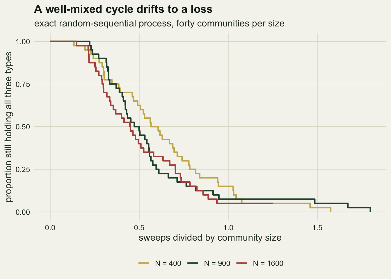
Small neighbourhoods keep all three types
side_main   <- 40
n_lat       <- 30
radius_main <- c(0, 1, 3)

set.seed(4102)
lat_runs <- lapply(radius_main, function(r) run_lattice(side_main, r, n_lat, max_sweep))

lat_tab <- as.data.frame(t(vapply(lat_runs, km_table, numeric(6))))
lat_tab$radius <- radius_main
lat_tab$nb     <- c(4, (2 * radius_main[-1] + 1)^2 - 1)
lat_lost_all   <- sum(lat_tab$lost)
lat_n_all      <- sum(lat_tab$n)
upper_95       <- 1 - 0.05^(1 / n_lat)
mixed_1600_by_end <- 1 - n_cens_big / n_mixed
spacing_main   <- 8
On a 40 by 40 lattice, 1600 sites and so the same size as the largest well-mixed community, none of the 90 runs with a von Neumann neighbourhood, a radius 1 square or a radius 3 square lost a type in 2000 sweeps. With no losses at all, every Kaplan-Meier curve stays at one and the median cannot be estimated; the honest summary is a bound. With zero losses in 30 runs, the one-sided 95 per cent upper limit on the probability that a run loses a type by sweep 2000 is 0.095 for each neighbourhood. The well-mixed community of the same size had lost a type by that time in 0.95 of its runs.
The neighbourhoods here hold 4, 8 and 48 sites. The lattice runs used classes on a sublattice of spacing 8, and the last section checks that batching. Where it compared a schedule with one closer to one event at a time (the well-mixed control and radius 7), the cruder schedule made loss come earlier; for the von Neumann neighbourhood no schedule tried produced a loss, and radius 1 and radius 3 were run on this lattice only with spacing 8.
This is the Kerr plate result in a model with none of the plate’s biology: no diffusion of colicin, no nutrients, no empty space. Local invasion alone is enough. A patch of type 1 advances into type 2 on one side and is eaten by type 3 on the other, so every type is always being lost somewhere and gained somewhere else, and the lattice holds many such fronts at different phases. A local loss of type 1 in one region is not a loss for the community, because type 1 is still advancing elsewhere.
lat_km <- rbind(
  do.call(rbind, lapply(seq_along(radius_main), function(i)
    km_df(lat_runs[[i]], c("von Neumann", "radius 1", "radius 3")[i]))),
  km_df(mixed_runs[[3]], "well mixed"))
lat_km <- rbind(lat_km, data.frame(time = max_sweep, surv = 1,
                                   group = c("von Neumann", "radius 1", "radius 3")))
lat_km$group <- factor(lat_km$group,
                       levels = c("von Neumann", "radius 1", "radius 3", "well mixed"))

ggplot(lat_km, aes(time, surv, colour = group, linetype = group)) +
  geom_step(linewidth = 0.9) +
  scale_colour_manual(values = c(te_forest, te_gold, te_body, te_rust), name = NULL) +
  scale_linetype_manual(values = c("solid", "dashed", "dotted", "solid"), name = NULL) +
  scale_y_continuous(limits = c(0, 1)) +
  labs(x = "sweeps", y = "proportion still holding all three types",
       title = "Small neighbourhoods keep the cycle",
       subtitle = "N = 1600; runs censored at two thousand sweeps") +
  theme_datasheet() +
  theme(legend.position = "bottom")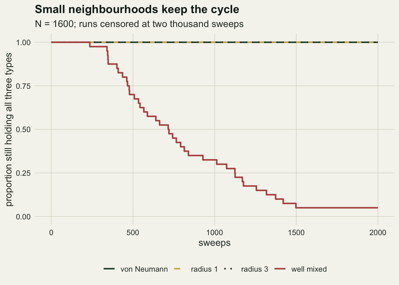
A wide neighbourhood keeps much less
wide_spacing <- 20
set.seed(4106)
trace_vn <- run_lattice(side_main, 0, 3, 300, trace_every = 1)
trace_r7 <- run_lattice(side_main, 7, 3, 300, trace_every = 1, min_spacing = wide_spacing)
trace_df <- rbind(cbind(trace_vn$trace, kernel = "von Neumann"),
                  cbind(trace_r7$trace, kernel = "radius 7"))
trace_df$kernel <- factor(trace_df$kernel, levels = c("von Neumann", "radius 7"))
window <- trace_df$sweep >= 30
amp <- tapply(trace_df$x1[window], trace_df$kernel[window], sd)

snap_sweep <- 150
set.seed(4108)
snap_vn <- run_lattice(side_main, 0, 1, snap_sweep, trace_every = snap_sweep)
snap_r7 <- run_lattice(side_main, 7, 1, snap_sweep, trace_every = snap_sweep,
                       min_spacing = wide_spacing)

set.seed(4111)
wide_run <- run_lattice(side_main, 7, n_lat, max_sweep, min_spacing = wide_spacing)
wide_tab <- km_table(wide_run)
test_wide <- survdiff(Surv(c(wide_run$time, mixed_runs[[3]]$time),
                           c(wide_run$lost, mixed_runs[[3]]$lost)) ~
                        rep(c("radius 7", "mixed"), c(n_lat, n_mixed)))
p_wide <- pchisq(test_wide$chisq, df = 1, lower.tail = FALSE)

set.seed(4103)
small_side   <- 20
small_radius <- c(1, 3, 9)
small_runs <- lapply(small_radius, function(r)
  run_lattice(small_side, r, n_lat, max_sweep, min_spacing = small_side))
small_tab <- as.data.frame(t(vapply(small_runs, km_table, numeric(6))))
small_tab$radius <- small_radius
small_nb <- (2 * small_radius + 1)^2 - 1
small_share <- small_nb / (small_side^2 - 1)
The snapshots show the difference in structure. After 150 sweeps the von Neumann lattice is a patchwork of single-type domains several sites across, with fronts between them. The radius 7 lattice, whose neighbourhood covers 224 sites, looks like salt and pepper: at that range each site draws its invader from a wide sample of the community, and domains do not form. The traces tell the same story in time. Past sweep 30 the standard deviation of the type 1 frequency is 0.085 on the von Neumann lattice, where the fronts are out of phase with each other and their contributions partly cancel, and 0.151 at radius 7, where the whole lattice cycles together and the oscillation grows.
A coherent oscillation behaves like the well-mixed cycle, so a wide neighbourhood keeps much less of the protection. Run to 2000 sweeps, 26 of 30 radius 7 lattices lost a type, with a median of 1312 sweeps (95 per cent interval 910 to 1851). That is later than the well-mixed community of the same size (log-rank p = 0.001), so a radius 7 neighbourhood does keep some structure, but it is nothing like the complete persistence of the smaller neighbourhoods. These radius 7 runs used finer batches than the rest of the lattice runs, spacing 20, for a reason the next section makes plain: batching pulls the radius 7 times down, so this median and this count of losses are more likely to understate persistence than to overstate it, and they are not an estimate of the exact schedule.
Whether a neighbourhood counts as local depends on the lattice as well as on the radius. On a 20 by 20 lattice, run one site at a time so that no batching is involved at all, a radius 1 neighbourhood lost a type in 18 of 30 runs (Kaplan-Meier median 1695 sweeps), radius 3 in 30 of 30 (median 298), and radius 9, whose neighbourhood is 0.90 of the lattice, in 30 of 30 with a median of 186 sweeps (95 per cent interval 154 to 239), an interval that overlaps the one for the well-mixed community of 400 individuals. The radius 1 neighbourhood that never lost a type in 30 runs on the larger lattice does lose one on this lattice: a lattice of this size holds too few domains for the out-of-phase averaging to work.
snap_grid <- data.frame(row = rep(seq_len(side_main), side_main),
                        col = rep(seq_len(side_main), each = side_main))
snap_df <- rbind(cbind(snap_grid, type = factor(snap_vn$state), kernel = "von Neumann"),
                 cbind(snap_grid, type = factor(snap_r7$state), kernel = "radius 7"))
snap_df$kernel <- factor(snap_df$kernel, levels = c("von Neumann", "radius 7"))

p_snap <- ggplot(snap_df, aes(col, row, fill = type)) +
  geom_raster() +
  facet_wrap(~ kernel) +
  coord_equal(expand = FALSE) +
  scale_fill_manual(values = c(te_forest, te_gold, te_rust), name = "type") +
  labs(x = NULL, y = NULL, title = "Domains against a well-mixed look") +
  theme_datasheet() +
  theme(axis.text = element_blank(), panel.grid.major = element_blank())

p_trace <- ggplot(trace_df, aes(sweep, x1, group = rep)) +
  geom_hline(yintercept = 1 / 3, linetype = "dashed", colour = te_rust, linewidth = 0.5) +
  geom_line(linewidth = 0.4, colour = te_ink, alpha = 0.6) +
  facet_wrap(~ kernel) +
  scale_y_continuous(limits = c(0, 1)) +
  labs(x = "sweeps", y = "frequency of type 1",
       subtitle = "three replicate lattices each; dashed red line at one third") +
  theme_datasheet()

(p_snap / p_trace) + plot_layout(heights = c(1.1, 1)) +
  plot_annotation(theme = theme_datasheet())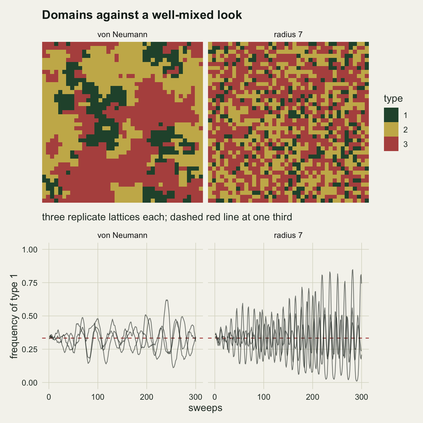
The update scheme can manufacture the answer
n_scheme <- 100
set.seed(4107)
scheme_exact   <- run_mixed(400, n_scheme, max_sweep)
scheme_batch   <- run_lattice(20, Inf, n_scheme, max_sweep, scheme = "batch")
scheme_permute <- run_lattice(20, Inf, n_scheme, max_sweep, scheme = "permute")
scheme_sync    <- run_lattice(20, Inf, n_scheme, max_sweep, scheme = "sync")

scheme_med <- vapply(list(scheme_exact, scheme_batch, scheme_permute, scheme_sync),
                     function(z) km_table(z)["median"], numeric(1))
test_batch <- survdiff(Surv(c(scheme_exact$time, scheme_batch$time),
                            c(scheme_exact$lost, scheme_batch$lost)) ~
                         rep(c("exact", "batch"), each = n_scheme))
p_batch <- pchisq(test_batch$chisq, df = 1, lower.tail = FALSE)
Every lattice result above rests on how events were scheduled, and a cyclic model is a sensitive place to get this wrong. Checking a spatial cooperation model found that the existence of cooperation in the prisoner’s dilemma survives a change from synchronous to asynchronous updating while the location of the collapse does not, following Huberman and Glance’s objection. Here the test is sharper, because the well-mixed community has an exact reference to compare against.
With the whole-lattice neighbourhood on 400 sites, four schedules of the same event were run 100 times each. The exact count process gave a median time to loss of 187 sweeps. The lattice engine with one site per class, which is random-sequential updating by construction, gave 190, and a log-rank test does not separate the two (p = 0.64); this is the check that the engine and the count process implement the same model. Visiting every site exactly once per sweep in a fresh random order, which is the loop many people write first, gave 20 sweeps. Updating the whole lattice at once from the previous state gave 22.
scheme_km <- rbind(km_df(scheme_exact, "exact, one event at a time"),
                   km_df(scheme_batch, "lattice engine, one site per class"),
                   km_df(scheme_permute, "each site once per sweep"),
                   km_df(scheme_sync, "whole lattice at once"))
scheme_km$group <- factor(scheme_km$group, levels = unique(scheme_km$group))
scheme_km$time  <- pmax(scheme_km$time, 1)
ggplot(scheme_km, aes(time, surv, colour = group, linetype = group)) +
  geom_step(linewidth = 0.9) +
  scale_x_log10(breaks = c(1, 10, 100, 1000), labels = c("1", "10", "100", "1000")) +
  scale_colour_manual(values = c(te_ink, te_forest, te_gold, te_rust), name = NULL) +
  scale_linetype_manual(values = c("dotted", "solid", "solid", "dashed"), name = NULL) +
  guides(colour = guide_legend(ncol = 2), linetype = guide_legend(ncol = 2)) +
  labs(x = "sweeps (log scale)", y = "proportion still holding all three types",
       title = "Scheduling changes the clock",
       subtitle = "N = 400, one hundred communities per scheme") +
  theme_datasheet() +
  theme(legend.position = "bottom", plot.margin = margin(6, 24, 6, 6))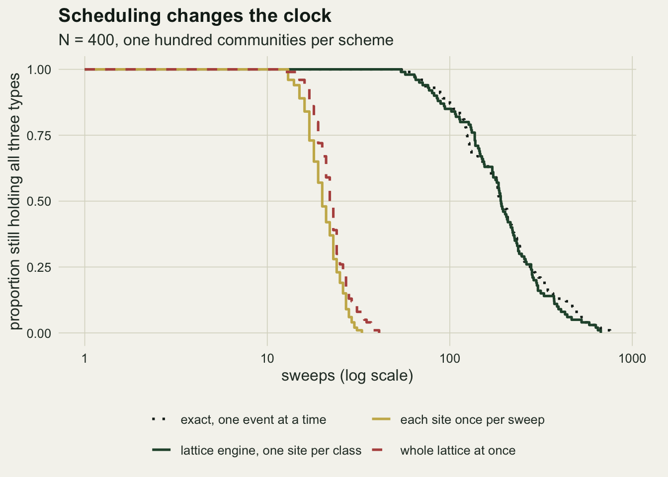
lump_spacing <- c(8, 10)
set.seed(4112)
lump_runs <- lapply(lump_spacing, function(s)
  run_lattice(side_main, 7, n_lat, max_sweep, min_spacing = s))
lump_runs[[3]] <- wide_run
lump_spacing <- c(lump_spacing, wide_spacing)
lump_classes <- lump_spacing^2
lump_med <- vapply(lump_runs, function(z) km_table(z)["median"], numeric(1))
test_lump <- survdiff(Surv(c(lump_runs[[1]]$time, wide_run$time),
                           c(lump_runs[[1]]$lost, wide_run$lost)) ~
                        rep(c("8", "20"), each = n_lat))
p_lump <- pchisq(test_lump$chisq, df = 1, lower.tail = FALSE)
test_coarse <- survdiff(Surv(c(lump_runs[[1]]$time, mixed_runs[[3]]$time),
                             c(lump_runs[[1]]$lost, mixed_runs[[3]]$lost)) ~
                          rep(c("radius 7", "mixed"), c(n_lat, n_mixed)))
p_coarse <- pchisq(test_coarse$chisq, df = 1, lower.tail = FALSE)
omega_sq <- 1 / 3
efold_lump <- 2 * lump_classes / omega_sq

like_share <- function(state, side, n_rep) {
  arr <- array(state, c(side, side, n_rep))
  right <- arr[, c(2:side, 1), , drop = FALSE]
  down  <- arr[c(2:side, 1), , , drop = FALSE]
  apply((arr == right) + (arr == down), 3, sum) / (2 * side * side)
}
one_at_a_time <- function(side, n_sweep) {
  n_cell <- side * side
  st   <- sample.int(3, n_cell, TRUE)
  n_ev <- n_cell * n_sweep
  tg   <- sample.int(n_cell, n_ev, TRUE)
  way  <- sample.int(4, n_ev, TRUE)
  for (e in seq_len(n_ev)) {
    i  <- tg[e] - 1
    rr <- i %% side
    cc <- i %/% side
    w  <- way[e]
    if (w == 1) rr <- (rr + 1) %% side else if (w == 2) rr <- (rr - 1) %% side else
      if (w == 3) cc <- (cc + 1) %% side else cc <- (cc - 1) %% side
    s_type <- st[cc * side + rr + 1]
    if (st[tg[e]] == beaten_by(s_type)) st[tg[e]] <- s_type
  }
  st
}
pattern_sweep <- 200
n_pat <- 12
set.seed(4109)
pat <- list(
  batch   = like_share(run_lattice(side_main, 0, n_pat, pattern_sweep,
                                   trace_every = pattern_sweep)$state, side_main, n_pat),
  permute = like_share(run_lattice(side_main, 0, n_pat, pattern_sweep, scheme = "permute",
                                   trace_every = pattern_sweep)$state, side_main, n_pat),
  sync    = like_share(run_lattice(side_main, 0, n_pat, pattern_sweep, scheme = "sync",
                                   trace_every = pattern_sweep)$state, side_main, n_pat),
  single  = vapply(seq_len(n_pat), function(i)
    like_share(one_at_a_time(side_main, pattern_sweep), side_main, 1), numeric(1)))
pat_mean <- vapply(pat, mean, numeric(1))
pat_se   <- vapply(pat, function(v) sd(v) / sqrt(length(v)), numeric(1))
pat_z    <- (pat_mean - pat_mean["single"]) / sqrt(pat_se^2 + pat_se["single"]^2)

set.seed(4110)
sync_vn <- run_lattice(side_main, 0, n_pat, max_sweep, scheme = "sync")
perm_vn <- run_lattice(side_main, 0, n_pat, max_sweep, scheme = "permute")
Both of the fast schedules introduce a delay. Under synchronous updating every event reads the state of the previous sweep. Under the once-per-sweep order a site that has already been visited cannot be invaded again until the next sweep, so the types that were growing at the start of the sweep keep their gains, and the dynamics respond to the frequencies with a lag of up to one sweep. A neutral cycle with a lag is no longer neutral: the explicit Euler step of a rotation spirals outwards, the amplitude grows, and the community runs into the boundary within a few cycles. The random-sequential median is 9.5 times the once-per-sweep median, and in both fast schedules the change is towards earlier loss.
The same effect enters through the batches of the lattice engine, more quietly. A class is exact as a set of events, but the events it groups are forbidden from seeing each other, whereas random targets in the same stretch of time would sometimes fall in each other’s neighbourhood and respond to each other’s changes. Where nearby regions of the lattice are out of phase with each other, as in the von Neumann domains, that costs little. When the whole lattice oscillates together, as it does at radius 7, one class is a small synchronous step of the coherent cycle. The linearised replicator cycle turns at an angular rate whose square is one third per sweep squared, and an Euler step of one class, a fraction one over the number of classes of a sweep, makes the amplitude grow by a factor e in about 384 sweeps with 64 classes, 600 with 100 and 2400 with 400. That is a rough scale, not a prediction of the time to loss, but it is the right order. Radius 7 on the 40 by 40 lattice gave median times to loss of 540, 672 and 1312 sweeps at those three batch sizes (log-rank p for the coarsest against the finest < 0.001). With the coarsest batching, which is the one the small neighbourhoods used, radius 7 would have been reported as losing a type faster than a well-mixed community of the same size (log-rank p = 0.008), the opposite of what the finest batching shows. That ranking is produced by the schedule. The finest batching affordable here may still carry some of the same bias, so its radius 7 median is more likely too short than too long.
For the small neighbourhoods the schedule changes the picture only slightly. After 200 sweeps on the von Neumann lattice, the share of neighbouring pairs holding the same type was 0.729 under true one-event-at-a-time updating (standard error 0.005, 12 lattices), 0.749 under the batched engine, 0.752 under synchronous updating and 0.782 under the once-per-sweep order. Those are 3.1, 3.2 and 7.8 standard errors above the one-at-a-time value: every shortcut makes the domains a little coarser, and the once-per-sweep order does so most. None of it touches persistence. Run to 2000 sweeps, 0 of 12 synchronous von Neumann lattices and 0 of 12 once-per-sweep lattices lost a type.
What to report
Report the event and the clock in words a reader could code: what is picked, from where, what happens, and how many events make a unit of time. Here that is a random target, a random source from the neighbourhood, replacement if the source wins, and one sweep per site. The mean-field limit of the rule is then known, and a reader can tell which deterministic model the simulation is the finite version of.
Name the update schedule, and check it against a one-event-at-a-time run on something small. For a neutral cycle the choice between random-sequential, once-per-sweep and synchronous updating moved the well-mixed median from 190 to 20 sweeps, and batch size alone moved a lattice median by a factor of 2.4. A persistence result that holds under every schedule, as the small neighbourhoods did, is safe to report; a rate, a median or a ranking of neighbourhoods needs the schedule stated and tested.
Treat time to first loss as a censored survival time. Give the run length, the number of runs that reached it, and Kaplan-Meier medians with intervals where they exist. Where no run lost a type the median does not exist, and the useful number is an upper confidence limit on the loss probability for that run length, which with 30 runs is 0.095.
Give the neighbourhood together with the lattice size. A radius 1 neighbourhood was local on 40 by 40 sites and not on 20 by 20, and in a field study the equivalent statement is the interaction distance relative to the extent of the habitat.
Honest limits
The model has no empty sites, no birth and death as separate events, and no movement. Reichenbach, Mobilia and Frey (2006) analysed the well-mixed version of a model with empty space in which reproduction and competition are distinct, and in its spatial version (Reichenbach, Mobilia and Frey 2007) mobility above a threshold destroys coexistence even on a large lattice; that threshold has no counterpart here because nothing moves. What this post shows is the simplest version of the effect, local invasion against global invasion with everything else fixed, and not the behaviour of any particular microbial or plant system.
The lattices are small. With 1600 sites the persistence of the small neighbourhoods was measured over 2000 sweeps, which is long against the well-mixed times but says nothing about much longer runs; a lattice of this size could in principle still lose a type through a rare coarsening event. The 20 by 20 runs show that the protection does erode as the lattice shrinks, and the post does not locate the size at which it sets in for each radius.
The radius 7 result is only partly resolved. The median moved from 540 to 1312 sweeps as the batches were refined, and the one-site-per-class schedule that is exact would have taken too long on this machine at that radius. The mechanism and the trend both point to the remaining bias running towards shorter times, but its size is not known.
The well-mixed scaling rests on three community sizes, and the log-log slope of 0.81 has no interval attached. The claim in the post is that the time to loss grows with community size at roughly half a sweep per individual over this range, not an estimate of an exponent.
Neighbourhoods were squares with wrapped edges and a von Neumann cross. Real habitats have edges, and at an edge a site has fewer neighbours and a front can pin. The type labels are also perfectly symmetric: every type beats the next at the same rate. Unequal invasion rates move the centre of the cycle away from one third each and change which type is lost first, and the comparison between local and global neighbourhoods would need to be run again for that case.
References
Kerr B, Riley MA, Feldman MW, Bohannan BJM 2002 Nature 418(6894):171-174 (10.1038/nature00823)
Reichenbach T, Mobilia M, Frey E 2006 Physical Review E 74(5):051907 (10.1103/PhysRevE.74.051907)
Reichenbach T, Mobilia M, Frey E 2007 Nature 448(7157):1046-1049 (10.1038/nature06095)
Sinervo B, Lively CM 1996 Nature 380(6571):240-243 (10.1038/380240a0)
Huberman BA, Glance NS 1993 Proceedings of the National Academy of Sciences 90(16):7716-7718 (10.1073/pnas.90.16.7716)