library(ggplot2)
library(patchwork)
library(MASS)

te_paper  <- "#f5f4ee"
te_ink    <- "#16241d"
te_body   <- "#2c3a31"
te_forest <- "#275139"
te_rust   <- "#b5534e"
te_gold   <- "#c9b458"
te_line   <- "#dad9ca"

theme_datasheet <- function() {
  theme_minimal(base_size = 12) +
    theme(plot.background  = element_rect(fill = te_paper, colour = NA),
          panel.background = element_rect(fill = te_paper, colour = NA),
          panel.grid.major = element_line(colour = te_line, linewidth = 0.3),
          panel.grid.minor = element_blank(),
          text             = element_text(colour = te_body),
          plot.title       = element_text(colour = te_ink, face = "bold"),
          plot.subtitle    = element_text(colour = te_body),
          axis.text        = element_text(colour = te_body))
}Likert items: when group means lie
R
questionnaires
ordinal data
human dimensions
simulation
MASS
ecology tutorial
A polarised stakeholder group can score lower on a 1 to 5 item with the same mean attitude. Simulating in R how t tests and polr fail, and a scale model holds.
A national park runs a questionnaire at its visitor centres and in the villages around it. One statement reads “Wolves should be protected in this region”, scored from 1 (strongly disagree) to 5 (strongly agree). Two hundred forms come back: a hundred from park visitors and a hundred from local farmers and hunters. The visitors average above four; the farmers and hunters average lower, a t test on the codes says the gap is significant, and the report to the steering group says that local residents are less supportive of wolf protection than visitors.
That sentence can be false even when the two groups hold exactly the same average attitude. The farmers and hunters are not uniformly lukewarm; they are split, with some strongly against wolves and some strongly for them. On a scale where most people tick “agree” or “strongly agree”, a wider spread of attitude empties the “agree” box in both directions. Those who move up can only reach “strongly agree”, one step higher; those who move down fall two or three steps to the disagree boxes. The code mean falls although the attitude mean has not moved. Liddell and Kruschke 2018 showed this class of failure for metric models applied to ordinal data, both false alarms and inversions of the sign of a real difference, and Buerkner and Vuorre 2019 give the ordinal models that avoid it. This post is a demonstration of their result in a survey setting, with rejection rates measured rather than illustrated, and with the model that repairs it written out by hand.
The ordinal model already on this site does not repair it on its own. Ordinal regression for ordered cover classes argues, correctly, that class codes are labels and that a linear model on them predicts “a phantom fractional class”; it fits a proportional odds model and presents that as the fix. It never meets two groups with different spreads, and a proportional odds model fitted with MASS::polr assumes one latent spread for everyone, so it is exposed to the same trap. Checking a bounded-response model tests the parallel slopes assumption with Brant’s test, which compares slopes across thresholds; a difference in latent spread is a different departure, and that test is not built for it. Observer agreement and Cohen’s kappa treats ordered classes as a question of agreement between two observers, not of comparing two groups. What this post adds is the measured error rate of the four usual analyses of a group comparison on a Likert item, and one extra parameter, a group scale, that brings the error rate back to nominal.
A latent attitude cut into five boxes
The generating model is the latent variable reading of an ordinal item (McCullagh 1980). Each respondent carries an attitude on a continuous scale; answering the item adds a little noise; four fixed thresholds cut the result into five boxes. Visitors have attitude mean zero and standard deviation one. Farmers and hunters have the same mean in the null scenario, and a standard deviation of 2.2. The thresholds sit low on the scale, so that most visitors agree. All of these values were fixed before any rate was computed.
tau      <- c(-2.2, -1.5, -0.8, 0.1)   # thresholds between the five boxes
noise_sd <- 0.6                        # answering noise per item
n_grp    <- 100                        # respondents per group
sd_polar <- 2.2                        # latent SD of farmers and hunters
mu_shift <- 0.4                        # real latent shift in the second scenario
k_cat    <- 5
alpha_lev <- 0.05; z_crit <- qnorm(1 - alpha_lev / 2)
sd_tot_ref <- sqrt(1 + noise_sd^2)     # visitors: attitude plus answering noise

to_box <- function(z) findInterval(z, tau) + 1L
box_prob <- function(mu, s, cuts = tau) diff(c(0, pnorm((cuts - mu) / s), 1))

gam_shape <- 4                         # skewed check: gamma attitude with this shape
draw_group <- function(n, mu, s, items, camps = FALSE, skew = 0) {
  att <- if (camps) sample(c(-1, 1), n, TRUE) * sqrt(s^2 - 1) + rnorm(n) + mu
         else if (skew != 0) mu + skew * s * (rgamma(n, gam_shape) - gam_shape) / sqrt(gam_shape)
         else rnorm(n, mu, s)
  matrix(to_box(rep(att, items) + rnorm(n * items, 0, noise_sd)), nrow = n)
}

set.seed(2417)
ex_vis  <- draw_group(n_grp, 0, 1, 1)[, 1]
ex_farm <- draw_group(n_grp, 0, sd_polar, 1)[, 1]
ex_tab  <- rbind(visitors = tabulate(ex_vis, k_cat), farmers = tabulate(ex_farm, k_cat))
colnames(ex_tab) <- 1:k_cat
ex_tab
1 2 3 4 5
visitors 1 7 13 34 45
farmers 13 12 14 16 45ex_t <- t.test(ex_farm, ex_vis)
ex_w <- suppressWarnings(wilcox.test(ex_farm, ex_vis))In this one survey the visitors average 4.15 and the farmers and hunters 3.68. Welch’s t test on the codes gives p = 0.0083 and the Wilcoxon rank sum test p = 0.097. The table shows where the difference comes from: 25 farmers and hunters in the two disagree boxes against 8 visitors, while the “strongly agree” box, the only place the upper half of the extra spread can go, holds 45 farmers and hunters against 45 visitors.
The population code means have a closed form, because the probability of each box is a difference of two normal distribution functions. Each group’s answer is its attitude plus noise, so the spread that meets the thresholds is the square root of the attitude variance plus the noise variance.
code_moments <- function(mu, s, cuts = tau) {
  p <- box_prob(mu, sqrt(s^2 + noise_sd^2), cuts)
  m <- sum(p * seq_along(p)); c(mean = m, var = sum(p * seq_along(p)^2) - m^2)
}
welch_power <- function(mu, s, n = n_grp) {
  a <- code_moments(0, 1); b <- code_moments(mu, s)
  gap <- b[["mean"]] - a[["mean"]]; se <- sqrt(a[["var"]] / n + b[["var"]] / n)
  c(gap = gap, reject = pnorm(-z_crit - gap / se) + pnorm(-z_crit + gap / se),
    lower = pnorm(-z_crit - gap / se))
}
# probability that a random farmer answers higher than a random visitor, ties halved
superiority <- function(mu, s) {
  p0 <- box_prob(0, sd_tot_ref); p1 <- box_prob(mu, sqrt(s^2 + noise_sd^2))
  sum(outer(p1, p0) * (outer(1:k_cat, 1:k_cat, ">") + 0.5 * (outer(1:k_cat, 1:k_cat, "=="))))
}
cm_ref <- code_moments(0, 1)[["mean"]]
cm_pol <- code_moments(0, sd_polar)[["mean"]]
cm_shift <- code_moments(mu_shift, sd_polar)[["mean"]]
pw_null <- welch_power(0, sd_polar); pw_shift <- welch_power(mu_shift, sd_polar)
sup_null <- superiority(0, sd_polar)
With identical attitude means, the population code mean is 4.091 for visitors and 3.697 for farmers and hunters. Give the farmers and hunters a real attitude advantage of 0.4 and their code mean is still only 3.923, below the visitors. The Wilcoxon test is exposed too, less directly: the probability that a random farmer or hunter ticks a higher box than a random visitor, with ties counted as half, is 0.457 rather than one half, because the two attitude distributions are symmetric about the same centre but the boxes are not.
zz <- seq(-7, 7, length.out = 600)
dens <- rbind(data.frame(z = zz, d = dnorm(zz, 0, sd_tot_ref), group = "visitors"),
              data.frame(z = zz, d = dnorm(zz, 0, sqrt(sd_polar^2 + noise_sd^2)),
                         group = "farmers and hunters"))
grp_lev <- c("visitors", "farmers and hunters")
dens$group <- factor(dens$group, levels = grp_lev)
p_lat <- ggplot(dens, aes(z, d, colour = group)) +
  geom_vline(xintercept = tau, colour = te_body, linetype = "dashed", linewidth = 0.4) +
  geom_line(linewidth = 1) +
  scale_colour_manual(values = c(te_forest, te_rust), name = NULL) +
  labs(x = "attitude plus answering noise", y = "density",
       title = "Same centre, different spread",
       subtitle = "dashed lines: the four thresholds") +
  theme_datasheet() + theme(legend.position = "bottom")
bars <- data.frame(box = factor(rep(1:k_cat, 2)),
                   prob = c(box_prob(0, sd_tot_ref), box_prob(0, sqrt(sd_polar^2 + noise_sd^2))),
                   group = factor(rep(grp_lev, each = k_cat), levels = grp_lev))
p_box <- ggplot(bars, aes(box, prob, fill = group)) +
  geom_col(position = position_dodge(width = 0.75), width = 0.7) +
  scale_fill_manual(values = c(te_forest, te_rust), name = NULL) +
  labs(x = "box ticked (5: strongly agree)", y = "probability",
       title = "What the form records",
       subtitle = "population box probabilities") +
  theme_datasheet() + theme(legend.position = "bottom")
p_lat + p_box + plot_annotation(theme = theme_datasheet())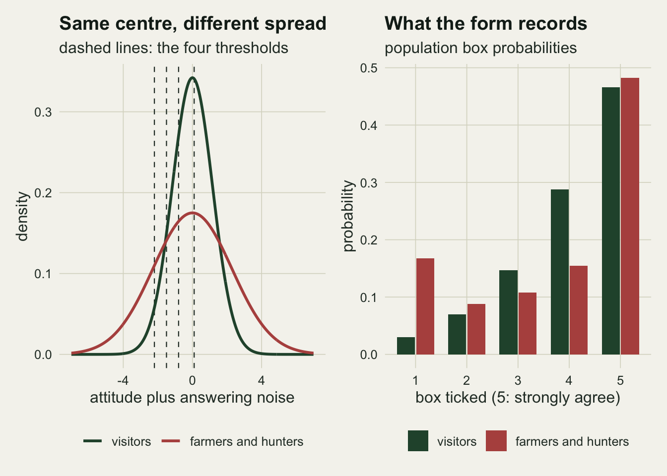
An ordered probit with a scale for each group
The cumulative probit model that MASS::polr fits with method = "probit" gives each group its own location on the latent scale and one shared spread. The extension needed here is one more parameter: a standard deviation for the second group, with the visitors fixing the unit (McCullagh 1980 wrote the location and scale model in this form; Agresti 2010 discusses location-scale cumulative link models). polr has no scale term, so the likelihood is written out below.
For a single item the likelihood depends on the data only through the two rows of box counts, so it is ten numbers whatever the sample size. The thresholds are parameterised as a first cut plus positive increments, the analytic gradient is supplied, and the Wald test of the location difference uses the Hessian. With several items per respondent the same marginal likelihood is used for every answer, and the standard error is a sandwich clustered on respondent, because six answers from one person are not six independent pieces of information.
group_score <- function(cuts, m, s, cnt) {
  zc <- (cuts - m) / s; fz <- dnorm(zc)
  p <- pmax(diff(c(0, pnorm(zc), 1)), 1e-300)
  r <- cnt[1:4] / p[1:4] - cnt[2:5] / p[2:5]
  list(gc = fz * r / s, gm = -sum(fz * r) / s, gls = -sum(fz * r * zc))
}
op_nll <- function(par, tab, free_scale) {
  cuts <- cumsum(c(par[1], exp(par[2:4]))); s <- if (free_scale) exp(par[6]) else 1
  p0 <- box_prob(0, 1, cuts); p1 <- box_prob(par[5], s, cuts)
  -sum(tab[1, ] * log(pmax(p0, 1e-300))) - sum(tab[2, ] * log(pmax(p1, 1e-300)))
}
op_score <- function(par, tab, free_scale) {
  cuts <- cumsum(c(par[1], exp(par[2:4]))); s <- if (free_scale) exp(par[6]) else 1
  a <- group_score(cuts, 0, 1, tab[1, ]); b <- group_score(cuts, par[5], s, tab[2, ])
  gc <- a$gc + b$gc
  c(sum(gc), exp(par[2:4]) * rev(cumsum(rev(gc)))[2:4], b$gm, if (free_scale) b$gls)
}
op_grad <- function(par, tab, free_scale) -op_score(par, tab, free_scale)

fit_ordered <- function(tab, free_scale = TRUE, person = NULL) {
  cum <- pmin(pmax(cumsum(colSums(tab))[1:4] / sum(tab), 0.01), 0.99)
  st0 <- qnorm(cum)
  start_par <- c(st0[1], log(pmax(diff(st0), 0.05)), 0, if (free_scale) 0)
  o <- optim(start_par, op_nll, op_grad, tab = tab, free_scale = free_scale, method = "BFGS")
  hess <- optimHess(o$par, op_nll, op_grad, tab = tab, free_scale = free_scale)
  vc <- tryCatch(solve(hess), error = function(e) NULL)
  if (is.null(vc)) return(c(est = o$par[5], se = NA, log_scale = NA, conv = 1))
  if (!is.null(person)) {
    np <- length(o$par); unit <- array(0, c(2, k_cat, np))
    for (gi in 1:2) for (j in 1:k_cat) {
      e <- matrix(0, 2, k_cat); e[gi, j] <- 1
      unit[gi, j, ] <- op_score(o$par, e, free_scale)
    }
    u <- rbind(person[[1]] %*% unit[1, , ], person[[2]] %*% unit[2, , ])
    vc <- vc %*% crossprod(u) %*% vc
  }
  c(est = o$par[5], se = sqrt(vc[5, 5]),
    log_scale = if (free_scale) o$par[6] else NA, conv = o$convergence)
}

ex_grp <- rep(0:1, each = n_grp); ex_y <- factor(c(ex_vis, ex_farm), levels = 1:k_cat)
polr_pr <- summary(polr(ex_y ~ ex_grp, method = "probit", Hess = TRUE))$coefficients["ex_grp", ]
own_eq  <- fit_ordered(ex_tab, free_scale = FALSE)
own_het <- fit_ordered(ex_tab, free_scale = TRUE)
chk_gap <- max(abs(c(own_eq[["est"]] - polr_pr[[1]], own_eq[["se"]] - polr_pr[[2]])))
p_polr_ex <- 2 * pnorm(-abs(polr_pr[[1]] / polr_pr[[2]]))
p_het_ex  <- 2 * pnorm(-abs(own_het[["est"]] / own_het[["se"]]))
With the scale fixed at one, the hand-coded fit is the probit polr model, and on the example survey the two agree on the location difference and its standard error to 5.6e-07. That agreement is why the simulation below can use the fast count-based fit in place of polr itself. On the same survey polr puts the farmers and hunters 0.325 latent units below the visitors with p = 0.0388. The scale model estimates the difference at -0.143 with p = 0.580, and a standard deviation ratio of 1.97, against a true ratio of 1.96 once the answering noise is included.
Error rates over many surveys
Four analyses of the same simulated surveys: Welch’s t test on the codes (or on each respondent’s mean over the items), the Wilcoxon rank sum test on the same numbers, the equal-scale ordered probit that polr fits, and the ordered probit with a group scale. Two spreads, two true location differences, and a questionnaire with either one item or six items that measure the same attitude. That is eight scenarios; the number of surveys per scenario was set before any rate was seen.
A rejection is a survey with p < 0.05. A wrong-sign rejection is a rejection in which the estimated difference points the opposite way from the true one, and in the null scenarios, where there is no true direction, it counts rejections that call the farmers and hunters less supportive.
n_surv <- 1500
welch_p <- function(a, b) {
  va <- var(a) / length(a); vb <- var(b) / length(b)
  tt <- (mean(b) - mean(a)) / sqrt(va + vb)
  dfw <- (va + vb)^2 / (va^2 / (length(a) - 1) + vb^2 / (length(b) - 1))
  c(2 * pt(-abs(tt), dfw), sign(tt))
}
wilcox_p <- function(a, b) {   # normal approximation with ties and continuity correction
  x <- c(a, b); rk <- rank(x); na <- length(a); nb <- length(b); nt <- na + nb
  w <- sum(rk[(na + 1):nt]) - nb * (nb + 1) / 2 - na * nb / 2
  ties <- table(x)
  s_w <- sqrt(na * nb / 12 * ((nt + 1) - sum(ties^3 - ties) / (nt * (nt - 1))))
  c(2 * pnorm(-abs((w - sign(w) * 0.5) / s_w)), sign(w))
}
chk_w <- abs(wilcox_p(ex_vis, ex_farm)[1] - ex_w$p.value)
chk_t <- abs(welch_p(ex_vis, ex_farm)[1] - ex_t$p.value)

one_survey <- function(mu, s, items, camps = FALSE, skew = 0) {
  y0 <- draw_group(n_grp, 0, 1, items); y1 <- draw_group(n_grp, mu, s, items, camps, skew)
  tw <- welch_p(rowMeans(y0), rowMeans(y1)); ww <- wilcox_p(rowMeans(y0), rowMeans(y1))
  tab <- rbind(tabulate(y0, k_cat), tabulate(y1, k_cat))
  person <- if (items > 1) list(t(apply(y0, 1, tabulate, k_cat)),
                                t(apply(y1, 1, tabulate, k_cat))) else NULL
  eq <- fit_ordered(tab, FALSE, person); het <- fit_ordered(tab, TRUE, person)
  c(t_p = tw[1], t_s = tw[2], w_p = ww[1], w_s = ww[2],
    eq_p = 2 * pnorm(-abs(eq[["est"]] / eq[["se"]])), eq_est = eq[["est"]],
    het_p = 2 * pnorm(-abs(het[["est"]] / het[["se"]])), het_est = het[["est"]],
    het_ls = het[["log_scale"]], het_conv = het[["conv"]])
}
cells <- expand.grid(mu = c(0, mu_shift), s = c(1, sd_polar), items = c(1, 6))
set.seed(6020)
raw <- lapply(seq_len(nrow(cells)), function(i)
  t(replicate(n_surv, one_survey(cells$mu[i], cells$s[i], cells$items[i]))))

meth_lev <- c("t test on codes", "Wilcoxon", "equal-scale probit (polr)", "group-scale probit")
rate_tab <- do.call(rbind, lapply(seq_len(nrow(cells)), function(i) {
  r <- raw[[i]]; wrong_dir <- -1  # less supportive in both kinds of scenario
  rej <- cbind(r[, "t_p"], r[, "w_p"], r[, "eq_p"], r[, "het_p"]) < alpha_lev
  sgn <- cbind(r[, "t_s"], r[, "w_s"], sign(r[, "eq_est"]), sign(r[, "het_est"]))
  data.frame(mu = cells$mu[i], s = cells$s[i], items = cells$items[i],
             method = factor(meth_lev, levels = meth_lev),
             rate = colMeans(rej, na.rm = TRUE),
             wrong = colMeans(rej & sgn == wrong_dir, na.rm = TRUE),
             right = colMeans(rej & sgn == 1, na.rm = TRUE))
}))
rate_tab$mcse <- sqrt(rate_tab$rate * (1 - rate_tab$rate) / n_surv)
n_fail <- sum(vapply(raw, function(r) sum(r[, "het_conv"] != 0 | is.na(r[, "het_p"])), 0))
rt <- function(mu, s, items, k, what = "rate")
  rate_tab[[what]][rate_tab$mu == mu & rate_tab$s == s & rate_tab$items == items &
                   rate_tab$method == meth_lev[k]]
mcse_nom <- sqrt(alpha_lev * (1 - alpha_lev) / n_surv)
The vectorised t and Wilcoxon functions reproduce t.test and wilcox.test on the example survey to 3.5e-18. Over all 12000 scale-model fits, 0 failed to converge or returned a singular Hessian.
When both groups have the same spread and the same mean, all four analyses hold their level with one item: 0.041 for the t test, 0.043 for Wilcoxon, 0.043 for the equal-scale probit and 0.038 for the group-scale probit, with a Monte Carlo standard error of 0.006 near five per cent.
Widen the farmers’ and hunters’ spread to 2.2 and keep the means equal. The t test rejects in 0.543 of surveys, and 814 of those 814 rejections call the farmers and hunters less supportive. Wilcoxon rejects in 0.209, the polr probit in 0.333. The group-scale model rejects in 0.041, and its false alarms lean one way: 0.029 of surveys are rejections calling the farmers and hunters less supportive and 0.013 the reverse.
rate_tab$scen <- factor(sprintf("SD %s, shift %s", ifelse(rate_tab$s == 1, "1", "2.2"),
                                ifelse(rate_tab$mu == 0, "0", "+0.4")),
                        levels = c("SD 1, shift 0", "SD 2.2, shift 0", "SD 1, shift +0.4", "SD 2.2, shift +0.4"))
rate_tab$item_lab <- factor(ifelse(rate_tab$items == 1, "one item", "six-item scale"),
                            levels = c("one item", "six-item scale"))
ggplot(rate_tab, aes(scen, rate, fill = method)) +
  geom_hline(yintercept = alpha_lev, colour = te_body, linetype = "dashed", linewidth = 0.5) +
  geom_col(position = position_dodge(width = 0.8), width = 0.75) +
  geom_errorbar(aes(ymin = pmax(rate - 2 * mcse, 0), ymax = rate + 2 * mcse),
                position = position_dodge(width = 0.8), width = 0.25,
                linewidth = 0.4, colour = te_ink) +
  facet_wrap(~ item_lab, ncol = 1) +
  scale_fill_manual(values = c(te_rust, te_gold, te_line, te_forest), name = NULL) +
  guides(fill = guide_legend(nrow = 2)) +
  labs(x = NULL, y = "share of surveys with p < 0.05",
       title = "Rejection rates: false alarms and real shifts",
       subtitle = "farmers and hunters against visitors, 100 respondents each; dashed line: 0.05") +
  theme_datasheet() + theme(legend.position = "bottom",
                            axis.text.x = element_text(size = 9))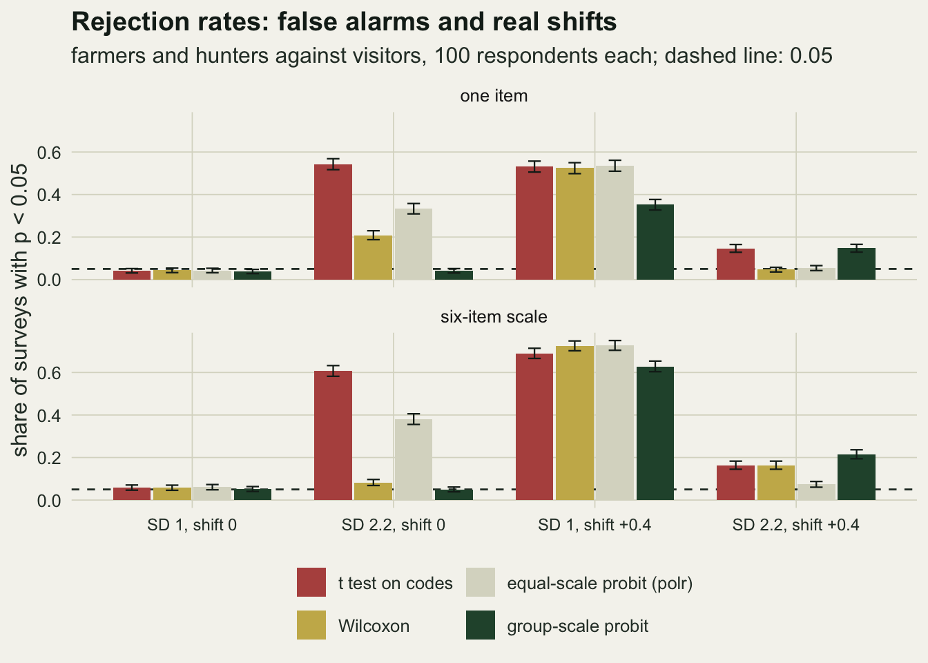
The t test arm is arithmetic
The t test result needs no simulation. Its rejection rate is the power of a two-sample comparison against the gap between the two population code means, and those means and variances were written down in closed form above. The normal approximation below ignores the Welch degrees of freedom, which at a hundred per group moves little.
t_sim_null  <- rt(0, sd_polar, 1, 1); t_sim_shift <- rt(mu_shift, sd_polar, 1, 1)
t_sim_shift_wrong <- rt(mu_shift, sd_polar, 1, 1, "wrong")
t_gap_null <- abs(t_sim_null - pw_null[["reject"]])
t_gap_shift <- abs(t_sim_shift_wrong - pw_shift[["lower"]])
mcse_t <- sqrt(t_sim_null * (1 - t_sim_null) / n_surv)
For equal means and a spread of 2.2, the closed form gives a rejection rate of 0.557 against 0.543 simulated, a gap of 0.014 with a Monte Carlo standard error of 0.013. With the real shift of 0.4 the closed form gives 0.151 for rejecting in the wrong direction against 0.145 simulated. So the t test is not unlucky here; it is correctly reporting that the code means differ. The code means are simply not the attitude means.
A real difference with the wrong sign
The scenario that should worry a steering group most has a real difference in it. The farmers and hunters really are more supportive on average, by 0.4 latent units, and still more polarised.
truth_std <- mu_shift / sd_tot_ref   # the shift on the visitors' answer scale
rev_i <- which(cells$mu == mu_shift & cells$s == sd_polar & cells$items == 1)
eq_mean <- mean(raw[[rev_i]][, "eq_est"]); het_mean <- mean(raw[[rev_i]][, "het_est"], na.rm = TRUE)
het_med <- median(raw[[rev_i]][, "het_est"], na.rm = TRUE)
eq_neg <- mean(raw[[rev_i]][, "eq_est"] < 0)
null_i <- which(cells$mu == 0 & cells$s == sd_polar & cells$items == 1)
scale_true <- sqrt(sd_polar^2 + noise_sd^2) / sd_tot_ref
ratio_q <- quantile(exp(raw[[null_i]][, "het_ls"]), c(0.1, 0.5, 0.9), na.rm = TRUE)
With one item the t test rejects in 0.147 of surveys and 0.145 of all surveys are rejections saying the farmers and hunters are less supportive. Wilcoxon rejects in the wrong direction in 0.014 and in the right direction in 0.033. The polr probit rejects in the wrong direction in 0.041, and its estimate is negative in 0.605 of surveys. The group-scale model rejects in the right direction in 0.147 and the wrong direction in 0.001.
On the visitors’ answer scale the true shift is 0.343. The group-scale estimate averages 0.381 (median 0.346); the equal-scale estimate averages -0.043, because with one shared spread the only way the model can put more farmers and hunters into the bottom boxes is to move their whole distribution down.
est_df <- rbind(data.frame(est = raw[[rev_i]][, "eq_est"], model = "equal-scale probit (polr)"),
                data.frame(est = raw[[rev_i]][, "het_est"], model = "group-scale probit"))
est_df$model <- factor(est_df$model, levels = meth_lev[3:4])
ggplot(est_df, aes(est, fill = model)) +
  geom_histogram(bins = 60, position = "identity", alpha = 0.75, colour = NA) +
  geom_vline(xintercept = truth_std, colour = te_ink, linetype = "dashed", linewidth = 0.8) +
  geom_vline(xintercept = 0, colour = te_body, linewidth = 0.4) +
  scale_fill_manual(values = c(te_rust, te_forest), name = NULL) +
  labs(x = "estimated difference, farmers and hunters minus visitors (latent units)",
       y = "surveys", title = "One shared spread drags the estimate to zero",
       subtitle = "dashed line: the true difference; solid line: zero") +
  theme_datasheet() + theme(legend.position = "bottom")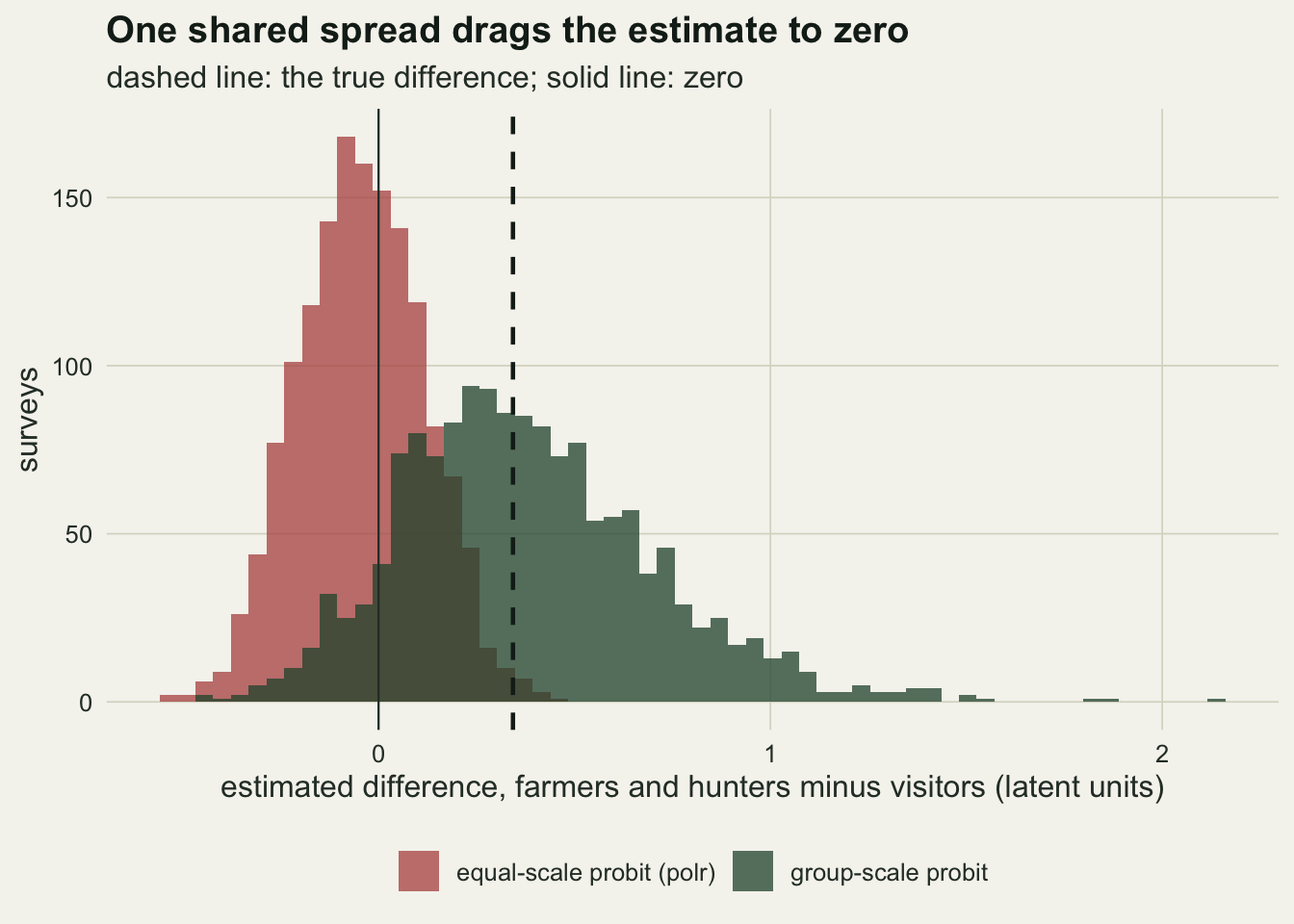
Six items do not rescue the mean
n_big <- 20000
set.seed(6022)
big0 <- rowMeans(draw_group(n_big, 0, 1, 6)); big1 <- rowMeans(draw_group(n_big, 0, sd_polar, 6))
rk_big <- rank(c(big0, big1))
sup_six <- (sum(rk_big[(n_big + 1):(2 * n_big)]) - n_big * (n_big + 1) / 2) / n_big^2
A standard response to a single noisy item is to ask several and average them. With six items that all measure the same attitude, the t test on respondent means rejects in 0.607 of null surveys, against 0.543 for one item: averaging removes answering noise, and the gap between the code means is still there. The equal-scale probit, with the same respondent-clustered sandwich, rejects in 0.381. The group-scale model with a respondent-clustered sandwich rejects in 0.050.
Wilcoxon behaves differently. The quantity it tests is the probability that a random farmer or hunter scores higher than a random visitor, ties halved, which was 0.457 for one item. A six-item mean is close to a smooth increasing function of each respondent’s attitude, and a rank test does not care how skewed that function is: an increasing map keeps the order of any two attitudes, so without ties and answering noise the probability would be exactly one half, because a random farmer’s or hunter’s attitude is as likely to lie above a random visitor’s as below it. Estimated from 20000 simulated respondents per group, the same probability for the six-item mean is 0.480. Its null rejection rate drops from 0.209 with one item to 0.083 with six. With the real shift, though, it rejects in the right direction in 0.161 of surveys against 0.215 for the group-scale model.
The extra parameter costs something when it is not needed. With equal spreads and a real shift, the t test detects the difference in 0.531 of one-item surveys and the group-scale model in 0.352; with six items the two rates are 0.690 and 0.629.
How polarised does a group have to be
The closed form makes it cheap to ask how the code-mean gap grows with the spread ratio, and whether the skewed thresholds matter. The symmetric thresholds below sit evenly around the visitors’ mean attitude.
tau_sym <- c(-1.5, -0.5, 0.5, 1.5)
sd_seq <- seq(1, 3, by = 0.05)
gap_at <- function(s, cuts) code_moments(0, s, cuts)[["mean"]] - code_moments(0, 1, cuts)[["mean"]]
sweep_df <- rbind(
  data.frame(s = sd_seq, gap = vapply(sd_seq, gap_at, 0, cuts = tau), cuts = "skewed"),
  data.frame(s = sd_seq, gap = vapply(sd_seq, gap_at, 0, cuts = tau_sym), cuts = "symmetric"))
break_even <- function(s) uniroot(function(m) code_moments(m, s)[["mean"]] - cm_ref, c(-2, 6))$root
be_seq <- seq(1, 3, by = 0.1)
be_df <- data.frame(s = be_seq, shift = vapply(be_seq, break_even, 0))
gap_15 <- gap_at(1.5, tau); gap_22 <- gap_at(sd_polar, tau); gap_sym_max <- max(abs(sweep_df$gap[sweep_df$cuts == "symmetric"]))
be_15 <- break_even(1.5); be_22 <- break_even(sd_polar)
pw_15 <- welch_power(0, 1.5)[["reject"]]
With symmetric thresholds the largest code-mean gap over spread ratios from one to three is 0.000: the extra spread fills both ends equally. With the skewed thresholds a spread of 1.5 already lowers the code mean by 0.189 boxes, and a t test at a hundred per group rejects in 0.199 of surveys; at 2.2 the code mean is lower by 0.394. For the code means to tie, the more polarised group needs a real attitude advantage of 0.27 latent units at a spread of 1.5 and 0.72 at 2.2.
p_gap <- ggplot(sweep_df, aes(s, gap, colour = cuts)) +
  geom_hline(yintercept = 0, colour = te_body, linewidth = 0.4) +
  geom_line(linewidth = 1) +
  scale_colour_manual(values = c(te_rust, te_forest), name = "thresholds") +
  labs(x = "latent SD, farmers and hunters", y = "code-mean gap (boxes)",
       title = "Equal attitude, unequal codes", subtitle = "same mean attitude in both groups") +
  theme_datasheet() + theme(legend.position = "bottom")
p_be <- ggplot(be_df, aes(s, shift)) +
  geom_line(linewidth = 1, colour = te_rust) + geom_point(size = 1.8, colour = te_rust) +
  labs(x = "latent SD, farmers and hunters", y = "latent advantage (units)",
       title = "Break-even advantage", subtitle = "skewed thresholds; code means equal") +
  theme_datasheet()
p_gap + p_be + plot_annotation(theme = theme_datasheet())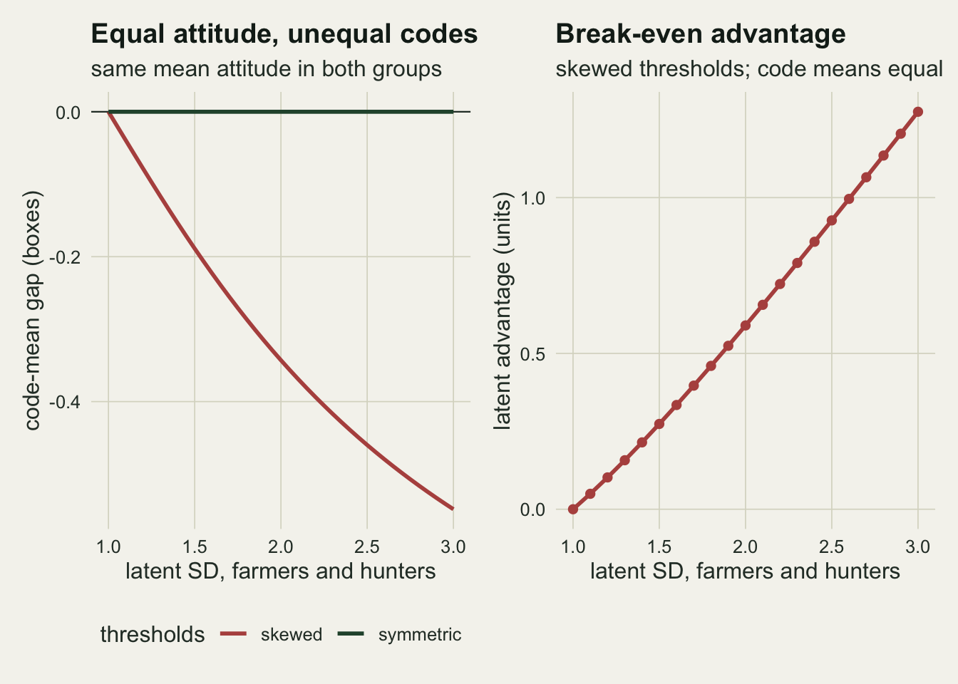
Two camps and a skewed attitude
A group described as polarised may not have a wide bell-shaped attitude distribution at all. It may be two camps. The scale model assumes a normal latent attitude in each group, so the fair test is to break that assumption: the farmers and hunters below are an even mix of two camps with the same total spread of 2.2 and the same mean as the visitors.
set.seed(6021)
camp_raw <- t(replicate(n_surv, one_survey(0, sd_polar, 1, camps = TRUE)))
camp_het <- mean(camp_raw[, "het_p"] < alpha_lev, na.rm = TRUE)
camp_t <- mean(camp_raw[, "t_p"] < alpha_lev)
camp_eq <- mean(camp_raw[, "eq_p"] < alpha_lev)
camp_centre <- sqrt(sd_polar^2 - 1)
# the model fitted to the exact box probabilities of the two-camp group (large counts)
p_camp <- 0.5 * (box_prob(-camp_centre, sqrt(1 + noise_sd^2)) + box_prob(camp_centre, sqrt(1 + noise_sd^2)))
big_tab <- 1e6 * rbind(box_prob(0, sd_tot_ref), p_camp)
fit_par <- optim(c(-2, log(c(0.5, 0.5, 0.8)), 0, 0), op_nll, op_grad, tab = big_tab,
                 free_scale = TRUE, method = "BFGS", control = list(maxit = 1000))$par
fit_cuts <- cumsum(c(fit_par[1], exp(fit_par[2:4])))
camp_misfit <- max(abs(c(box_prob(0, 1, fit_cuts) - box_prob(0, sd_tot_ref),
                         box_prob(fit_par[5], exp(fit_par[6]), fit_cuts) - p_camp)))
camp_loc <- fit_par[5]
box_se_max <- sqrt(max(c(p_camp, box_prob(0, sd_tot_ref)) * (1 - c(p_camp, box_prob(0, sd_tot_ref)))) / n_grp)
With camps centred at -1.96 and +1.96, the t test rejects in 0.811 of surveys, the polr probit in 0.551, and the group-scale model in 0.050. Fitted to the exact box probabilities of the two-camp group, the model returns a location difference of -0.014 and misses no box probability in either group by more than 0.026, while the sampling standard error of a box share at a hundred respondents is as large as 0.050. Five boxes cut through a two-camp attitude leave a pattern that a wide normal attitude reproduces to within that noise, so the one-item model neither detects the camps nor is misled by them in this mixture.
Both camps and the visitors’ bell curve are symmetric. A skewed attitude distribution is a different departure: a long tail of strong supporters with the peak of the group below the mean, or the mirror image, a long tail of strong opponents with the peak above it. Below, the farmers’ and hunters’ attitude is a gamma distribution with shape 4, shifted and rescaled to the visitors’ mean and the same spread of 2.2, once with the long tail to the right and once to the left. The box probabilities are integrated exactly, and a further set of surveys uses the right-skewed version.
skew_box <- function(mu, s, dir, cuts = tau) {
  cdf <- vapply(cuts, function(cc) integrate(function(g) dgamma(g, gam_shape) *
    pnorm((cc - mu - dir * s * (g - gam_shape) / sqrt(gam_shape)) / noise_sd),
    0, Inf, rel.tol = 1e-10)$value, 0)
  diff(c(0, cdf, 1))
}
fit_exact <- function(p1) {
  optim(c(-2, log(c(0.5, 0.5, 0.8)), 0, 0), op_nll, op_grad,
        tab = 1e6 * rbind(box_prob(0, sd_tot_ref), p1), free_scale = TRUE,
        method = "BFGS", control = list(maxit = 1000))$par
}
skew_r <- fit_exact(skew_box(0, sd_polar, 1)); skew_l <- fit_exact(skew_box(0, sd_polar, -1))
het_null_sd <- sd(raw[[null_i]][, "het_est"], na.rm = TRUE)
set.seed(6023)
skew_raw <- t(replicate(n_surv, one_survey(0, sd_polar, 1, skew = 1)))
skew_rej <- mean(skew_raw[, "het_p"] < alpha_lev, na.rm = TRUE)
skew_low <- mean(skew_raw[, "het_p"] < alpha_lev & skew_raw[, "het_est"] < 0, na.rm = TRUE)
skew_t <- mean(skew_raw[, "t_p"] < alpha_lev)
Fitted to the exact box probabilities, the group-scale model puts the right-skewed group -0.257 latent units from the visitors, with a scale ratio of 1.68, and the left-skewed group at +0.323, with a ratio of 2.16; the true difference is zero in both. For comparison, the standard deviation of the location estimate over the one-item null surveys above is 0.283. In the simulated surveys with the right-skewed group the scale model rejects in 0.237 of surveys, and 0.237 of all surveys are rejections calling the farmers and hunters less supportive, against 0.041 when the attitude is normal; the t test rejects in 0.795. The scale model repairs a difference in spread, not a difference in shape.
Is the scale identified by one item
Two groups and five boxes give eight independent box probabilities. The group-scale model uses four thresholds, a location and a scale, six parameters in all, so a single item does identify it, with two degrees of freedom to spare. The price is precision.
In the null surveys with the wider spread, the estimated standard deviation ratio has a median of 1.99 against a true 1.96, and its 10th and 90th percentiles are 1.58 and 2.54. The identification rests on two assumptions: the thresholds are shared, and the latent attitude has the shape the probit assumes in both groups. The section above shows that two symmetric camps do little harm here and a skewed attitude moves the location estimate. If visitors and farmers read the boxes differently, which is differential item functioning, each group has its own four thresholds, the model has more parameters than the eight box probabilities can carry, and location, scale and threshold shift cannot be separated from one item. Several items with some thresholds held common are the usual way out.
What to report
Report the full box counts for each group, not only the means. The table of counts is the sufficient statistic for a single item, it takes ten numbers, and a reader can see at once whether one group is piled into both ends.
If a group comparison on a Likert item or a summed scale is the point of the study, fit an ordinal model and let the spread differ between groups. Report the location difference on the latent scale with its interval, and report the scale ratio as a finding in its own right: a group that is more divided about wolves is a different management problem from a group that is uniformly less keen.
Say which group fixes the latent unit, and say that the thresholds are assumed common and the latent attitude normal in each group. Those assumptions are what make the comparison possible, and they are the ones a reviewer should be invited to question.
When a t test on codes has already been published, the counts are enough for an audit: refit them with a group scale and see whether the location difference survives once the spread is free.
Honest limits
The group-scale model here is fitted by maximum likelihood with Wald tests. Liddell and Kruschke 2018 use a Bayesian ordered probit with the same structure, and the error rates reported here are frequentist rates of a frequentist procedure; they say nothing about how a posterior interval behaves at a hundred respondents per group.
The six-item analysis uses the marginal likelihood of each answer and a respondent-clustered sandwich. It is valid for the location difference but it does not model the respondent attitude as a random effect, so it discards information that a joint item-response model would use, and a joint model would be expected to reach higher power than the six-item figures here; that was not measured. The six items are also identical in their thresholds, which real scales never are.
The thresholds are fixed and skewed, and the spread ratio of 2.2 is large. The closed-form sweep shows the effect is present at smaller ratios, but whether it matters in a given human-wildlife conflict survey depends on how far the box probabilities in the reference group are from symmetric, and that is visible in the data before any model is fitted.
Every scenario uses a hundred respondents per group and a normal answering noise. Larger samples make the t test’s false alarm more certain, not less, because the code-mean gap is a population quantity; smaller samples leave the scale model with a poorly estimated spread, and its calibration at smaller samples was not measured here.
The shape checks are one mixture with equal camps and one gamma shape in two mirror directions. They show that skew moves the location estimate; how far it moves for other shapes, for unequal camps, or when both groups are skewed, was not measured.
References
Liddell TM, Kruschke JK 2018 Journal of Experimental Social Psychology 79:328-348 (10.1016/j.jesp.2018.08.009)
Buerkner PC, Vuorre M 2019 Advances in Methods and Practices in Psychological Science 2(1):77-101 (10.1177/2515245918823199)
McCullagh P 1980 Journal of the Royal Statistical Society Series B 42(2):109-127 (10.1111/j.2517-6161.1980.tb01109.x)
Agresti A 2010 Analysis of Ordinal Categorical Data, 2nd edition (ISBN 978-0-470-08289-8)