library(ggplot2)
library(patchwork)
library(MASS)

te_paper  <- "#f5f4ee"
te_ink    <- "#16241d"
te_body   <- "#2c3a31"
te_forest <- "#275139"
te_rust   <- "#b5534e"
te_gold   <- "#c9b458"
te_line   <- "#dad9ca"

theme_datasheet <- function() {
  theme_minimal(base_size = 12) +
    theme(plot.background  = element_rect(fill = te_paper, colour = NA),
          panel.background = element_rect(fill = te_paper, colour = NA),
          panel.grid.major = element_line(colour = te_line, linewidth = 0.3),
          panel.grid.minor = element_blank(),
          text             = element_text(colour = te_body),
          plot.title       = element_text(colour = te_ink, face = "bold"),
          plot.subtitle    = element_text(colour = te_body),
          axis.text        = element_text(colour = te_body))
}Lasso, stepwise and the dropped confounder
R
regression
regularisation
causal inference
simulation
ecology tutorial
Choosing adjustment covariates by lasso or stepwise AIC drops a confounder the treatment then absorbs. Simulating in R why double selection repairs it.
A hundred upland pastures, a grazing intensity for each, and a pitfall-trap count of ground beetles. The question is whether grazing changes beetle activity, and the survey sheet carries twenty other site covariates: soil productivity, slope, moisture, altitude, pH, aspect and a list of things recorded because they were cheap to record. Nobody wants twenty adjustment terms in a model fitted to a hundred rows, so the covariates get chosen. Either a lasso picks them, with grazing kept out of the penalty because it is the effect of interest, or a backward stepwise search by AIC drops them one at a time with grazing forced to stay in. Whatever survives goes into an ordinary regression, and the grazing coefficient and its interval are reported.
Both routes choose covariates by how well they predict the beetles, and that is the flaw. Belloni, Chernozhukov and Hansen (2014, Review of Economic Studies) named it the failure of single selection and gave the repair, double selection: select covariates that predict the outcome, select covariates that predict the treatment, and adjust for the union. Leeb and Potscher 2005 had already set out why an interval computed after a data-driven choice of model cannot be read as if the model were fixed. This post is a demonstration of those results in an ecological design, not a claim to them. What it measures is where the rules an ecologist actually uses (the cross-validated lasso at its minimum, the one-standard-error lasso, backward AIC) sit between the failure and the repair, and in which design a lasso is worth using at all.
The site’s checking a penalised regression post shows what selection does to a coefficient it chose: a null predictor survives only on the datasets where its noise lined up with the response. Here the grazing coefficient is never penalised and never at risk of being dropped, and the penalty still sets its value through the covariates it throws away. The post on confounding and backdoor adjustment shows the bias of leaving a common cause out; here the common cause is recorded, offered to the model, and left out by the selection rule. And model-averaged coefficients shows the marginal slope drifting when a correlated covariate is omitted, with no selection rule and no treatment in the picture.
A hundred pastures, twenty covariates
Every simulated survey has the same structure. The twenty covariates are independent standard normals and all of them are measured before grazing is set. Soil productivity, x1, raises grazing intensity and raises beetle activity: it is the confounder. Slope, x2, is a second and weaker common cause. Moisture, altitude and pH (x3 to x5) drive the beetles and have nothing to do with grazing. The other fifteen covariates do nothing. Grazing itself has no effect, so the true value of its coefficient is zero, and any interval that excludes zero is wrong.
n_sites <- 100                        # pastures
p_main  <- 20                         # candidate covariates, all pre-treatment
a_graze <- c(0.8, 0.5)                # effects of x1 (productivity), x2 (slope) on grazing
b_main  <- 0.3                        # effect of the confounder x1 on beetles
b_rest  <- c(0.25, 1.0, 0.8, 0.5)     # effects of x2 to x5 on beetles
tau_0   <- 0                          # true grazing effect
n_rep   <- 400                        # replicates per cell, fixed before any rate was seen

make_sites <- function(n, p, b1 = b_main, tau = tau_0) {
  X <- matrix(rnorm(n * p), n, p); colnames(X) <- paste0("x", seq_len(p))
  graze <- as.numeric(X[, 1:2] %*% a_graze) + rnorm(n)
  y <- tau * graze + b1 * X[, 1] + as.numeric(X[, 2:5] %*% b_rest) + rnorm(n)
  list(X = X, graze = graze, y = y, folds = sample(rep(1:5, length.out = n)))
}
Grazing has variance 0.8^2 + 0.5^2 + 1 and the residual noise in both equations has variance one. All numbers below are for these fixed constants, chosen before anything was run.
Four ways to choose the covariates, written out
The lasso (Tibshirani 1996) is coded by hand, as in the site’s other penalised-regression posts, with the exact path from least angle regression with the lasso modification: lasso_path() follows the solution of (1 / 2n) ||y - Z b||^2 + lam ||b||_1 down from the largest penalty, and lasso_at() reads it off at any penalty. Grazing is kept out of the penalty by partialling it out first: regress the beetle count and every covariate on grazing, then run the lasso on the residuals. By the Frisch-Waugh-Lovell theorem this is exactly the lasso with an unpenalised grazing term, and a check below confirms it. For the cross-validated lasso each residualised covariate is divided by the spread of its raw column, which is how cv.glmnet standardises when grazing is given a zero penalty factor; the check is run on that scaling.
The plug-in penalty is the one Belloni, Chernozhukov and Hansen use (their 2014 Journal of Economic Perspectives paper sets it out): a penalty level of 2 c sqrt(n) qnorm(1 - gamma / (2 p)) with c = 1.1, and a loading for each covariate, the square root of the mean of the covariate squared times the residual squared, so a column with noisier residuals pays more. The residuals start from a least squares fit on the five covariates most correlated with the response and are refreshed from the least squares refit on the selected set until the loadings settle. The tail probability here is gamma = 0.1 / log(n); the cost of that choice is taken up further down.
standardise_cols <- function(X) {
  ctr <- colMeans(X); Xc <- sweep(X, 2, ctr)
  scl <- sqrt(colMeans(Xc^2))                 # n divisor, as glmnet
  list(Z = sweep(Xc, 2, scl, "/"), ctr = ctr, scl = scl)
}
# exact lasso path: minimise (1 / 2n) ||yc - Z b||^2 + lam ||b||_1, stopping once lam < lam_stop
lasso_path <- function(Z, yc, lam_stop = 0, eps = 1e-12) {
  n <- nrow(Z); p <- ncol(Z); b <- numeric(p); mu <- numeric(n)
  cr0 <- as.numeric(crossprod(Z, yc)); active <- which.max(abs(cr0))
  lam <- max(abs(cr0)) / n; B <- matrix(0, p, 1)
  if (lam[1] <= lam_stop) return(list(lam = lam, B = B))
  for (step in seq_len(4 * p)) {
    cr <- as.numeric(crossprod(Z, yc - mu)); cmax <- max(abs(cr[active]))
    sg <- sign(cr[active]); ZA <- sweep(Z[, active, drop = FALSE], 2, sg, "*")
    g1 <- as.numeric(solve(crossprod(ZA), rep(1, length(active))))
    aa <- 1 / sqrt(sum(g1)); w <- aa * g1
    u <- as.numeric(ZA %*% w); a <- as.numeric(crossprod(Z, u))
    idle <- setdiff(seq_len(p), active); j_in <- NA; gam <- cmax / aa
    if (length(idle)) {
      gp <- (cmax - cr[idle]) / (aa - a[idle]); gm <- (cmax + cr[idle]) / (aa + a[idle])
      gg <- pmin(ifelse(gp > eps, gp, Inf), ifelse(gm > eps, gm, Inf))
      if (min(gg) < gam) { gam <- min(gg); j_in <- idle[which.min(gg)] }
    }
    dirn <- sg * w; hit0 <- -b[active] / dirn; hit0[hit0 <= eps] <- Inf; j_out <- NA
    if (min(hit0) < gam) { gam <- min(hit0); j_out <- active[which.min(hit0)]; j_in <- NA }
    b[active] <- b[active] + gam * dirn; mu <- mu + gam * u; cmax <- cmax - gam * aa
    if (!is.na(j_out)) { b[j_out] <- 0; active <- setdiff(active, j_out) }
    if (!is.na(j_in)) active <- c(active, j_in)
    lam <- c(lam, max(cmax, 0) / n); B <- cbind(B, b)
    if (lam[length(lam)] <= lam_stop) break
    if (cmax <= 1e-10 * lam[1] * n || (is.na(j_in) && is.na(j_out))) break
  }
  list(lam = lam, B = B)
}
lasso_at <- function(path, lam_out) {         # linear interpolation along the exact path
  L <- path$lam; lam_out <- pmin(pmax(lam_out, min(L)), max(L))
  if (length(L) == 1) return(path$B[, rep(1, length(lam_out)), drop = FALSE])
  k <- pmin(pmax(findInterval(-lam_out, -L, rightmost.closed = TRUE), 1), length(L) - 1)
  wt <- (lam_out - L[k]) / (L[k + 1] - L[k]); wt[!is.finite(wt)] <- 0
  path$B[, k, drop = FALSE] + sweep(path$B[, k + 1, drop = FALSE] - path$B[, k, drop = FALSE], 2, wt, "*")
}
partial_out <- function(v, graze) {           # residuals of v on (1, graze)
  g_ctr <- graze - mean(graze); vc <- scale(as.matrix(v), scale = FALSE)
  vc - outer(g_ctr, colSums(vc * g_ctr) / sum(g_ctr^2))
}
# residualised columns divided by the spread of the RAW columns: the glmnet scaling with grazing unpenalised
standardise_raw <- function(X, graze) {
  scl <- sqrt(colMeans(sweep(X, 2, colMeans(X))^2))
  list(Z = sweep(partial_out(X, graze), 2, scl, "/"), scl = scl)
}
# plug-in lasso: penalty 2 c sqrt(n) qnorm(1 - gamma / (2p)) on the (1 / n) RSS scale, with loadings
c_pen <- 1.1; n_load_max <- 15
plugin_level <- function(n, p, gamma = 0.1 / log(n)) 2 * c_pen * sqrt(n) * qnorm(1 - gamma / (2 * p))
fit_lasso_plugin <- function(X, y) {
  n <- nrow(X); p <- ncol(X); Xc <- scale(X, scale = FALSE); yc <- y - mean(y)
  lam_std <- plugin_level(n, p) / (2 * n)     # the same penalty on the (1 / 2n) RSS scale
  top5 <- order(-abs(cor(Xc, yc)))[1:min(5, p)]
  e <- lm.fit(cbind(1, Xc[, top5]), yc)$residuals; psi_old <- rep(Inf, p)
  for (it in seq_len(n_load_max)) {
    psi <- sqrt(colMeans(Xc^2 * e^2))
    b <- lasso_at(lasso_path(sweep(Xc, 2, psi, "/"), yc, lam_std), lam_std)[, 1] / psi
    sel <- which(b != 0)
    e <- if (length(sel)) lm.fit(cbind(1, Xc[, sel]), yc)$residuals else yc
    if (max(abs(psi - psi_old)) < 1e-4) break
    psi_old <- psi
  }
  # lambda: the penalty per covariate on the standardised scale, for comparison with CV
  list(coef = b, lambda = lam_std * psi / sqrt(colMeans(Xc^2)), sel = sel, passes = it)
}
# five-fold CV lasso as cv.glmnet runs it: raw columns standardised, grazing unpenalised and
# refitted by least squares inside each fold
fit_lasso_cv <- function(X, y, graze, folds, n_lam = 40) {
  st <- standardise_raw(X, graze); full <- lasso_path(st$Z, partial_out(y, graze)[, 1])
  lams <- full$lam[1] * 10^seq(0, -3, length.out = n_lam)
  K <- max(folds); cv_err <- matrix(0, K, n_lam)
  for (k in seq_len(K)) {
    tr <- folds != k; gk <- graze[tr]
    s_k <- standardise_raw(X[tr, , drop = FALSE], gk)
    B_k <- lasso_at(lasso_path(s_k$Z, partial_out(y[tr], gk)[, 1]), lams) / s_k$scl
    r_k <- y[tr] - X[tr, , drop = FALSE] %*% B_k          # what is left for intercept and grazing
    g_k <- colSums(sweep(r_k, 2, colMeans(r_k)) * (gk - mean(gk))) / sum((gk - mean(gk))^2)
    a_k <- colMeans(r_k) - g_k * mean(gk)
    pred <- rep(a_k, each = sum(!tr)) + outer(graze[!tr], g_k) + X[!tr, , drop = FALSE] %*% B_k
    cv_err[k, ] <- colMeans((y[!tr] - pred)^2)
  }
  cvm <- colMeans(cv_err); cvs <- apply(cv_err, 2, sd) / sqrt(K)
  i_min <- which.min(cvm); i_1se <- min(which(cvm <= cvm[i_min] + cvs[i_min]))
  B <- lasso_at(full, lams[c(i_min, i_1se)]) / st$scl
  # lambda: median penalty per covariate on the partialled standardised scale, as for the plug-in
  to_partial <- median(st$scl / sqrt(colMeans(partial_out(X, graze)^2)))
  list(coef = B, lambda = lams[c(i_min, i_1se)] * to_partial,
       sel_min = which(B[, 1] != 0), sel_1se = which(B[, 2] != 0))
}
# backward elimination on n log(RSS / n) + 2 edf, the criterion stepAIC uses for lm; grazing forced in
back_aic <- function(X, y, graze) {
  n <- length(y); keep <- seq_len(ncol(X))
  aic_of <- function(k) { M <- cbind(1, graze, X[, k, drop = FALSE])
    n * log(sum(lm.fit(M, y)$residuals^2) / n) + 2 * ncol(M) }
  cur <- aic_of(keep)
  while (length(keep)) {
    cand <- vapply(seq_along(keep), function(i) aic_of(keep[-i]), 0)
    if (min(cand) >= cur) break
    cur <- min(cand); keep <- keep[-which.min(cand)]
  }
  keep
}
t_aic <- function(dfr, n = n_sites) sqrt(dfr * (exp(2 / n) - 1))   # |t| below which a drop lowers AIC
# the reported analysis: least squares of y on grazing plus the chosen covariates
ols_graze <- function(y, graze, Z = NULL) {
  M <- cbind(1, graze, Z); f <- lm.fit(M, y); dfr <- length(y) - ncol(M)
  s2 <- sum(f$residuals^2) / dfr; v22 <- chol2inv(qr.R(f$qr))[2, 2]
  c(est = unname(f$coefficients[2]), se = sqrt(s2 * v22), df = dfr)
}
Two of these are checked against an outside reference on one survey before anything is measured. The partialling route should give the same covariate coefficients as a lasso that carries grazing as an unpenalised column, solved here by plain coordinate descent on the raw columns standardised as glmnet standardises them, in which the grazing coefficient is updated by least squares and never thresholded. The hand-coded backward AIC should select the same set as MASS::stepAIC with grazing held in the lower scope.
set.seed(1207)
ex <- make_sites(n_sites, p_main)
st_ex <- standardise_raw(ex$X, ex$graze); lam_chk <- 0.05
b_fwl <- lasso_at(lasso_path(st_ex$Z, partial_out(ex$y, ex$graze)[, 1]), lam_chk)[, 1] / st_ex$scl

soft <- function(z, g) sign(z) * pmax(abs(z) - g, 0)
W  <- sweep(scale(ex$X, scale = FALSE), 2, st_ex$scl, "/")   # raw columns standardised, as glmnet does
g_ctr <- ex$graze - mean(ex$graze); res <- ex$y - mean(ex$y)
b_cd <- numeric(p_main); g_cd <- 0; w2 <- colMeans(W^2)
for (sweep_no in 1:100000) {
  b_old <- c(g_cd, b_cd)
  res <- res + g_ctr * g_cd; g_cd <- sum(g_ctr * res) / sum(g_ctr^2); res <- res - g_ctr * g_cd
  for (j in seq_len(p_main)) {
    res <- res + W[, j] * b_cd[j]
    b_cd[j] <- soft(mean(W[, j] * res), lam_chk) / w2[j]
    res <- res - W[, j] * b_cd[j]
  }
  if (max(abs(c(g_cd, b_cd) - b_old)) < 1e-13) break
}
gap_fwl <- max(abs(b_fwl - b_cd / st_ex$scl))

dd <- data.frame(y = ex$y, graze = ex$graze, ex$X)
sa <- stepAIC(lm(y ~ ., dd), scope = list(lower = ~ graze), direction = "backward", trace = 0)
set_mass <- setdiff(names(coef(sa)), c("(Intercept)", "graze"))
set_hand <- colnames(ex$X)[back_aic(ex$X, ex$y, ex$graze)]
same_set <- setequal(set_mass, set_hand)
The partialling route and coordinate descent with an unpenalised grazing column agree to \(9.4 \times 10^{-14}\) after 45 sweeps, and the hand-coded backward search and stepAIC keep exactly the same 5 covariates (x1, x2, x3, x4, x5).
One survey, five answers
On that one survey, each rule chooses its covariates and the same least squares fit is run on grazing plus whatever it chose. Double selection runs the plug-in lasso twice, once for beetles on the covariates and once for grazing on the covariates, and keeps the union.
sel_ex <- list(
  "plug-in single" = fit_lasso_plugin(partial_out(ex$X, ex$graze), partial_out(ex$y, ex$graze)[, 1])$sel,
  "CV min single"  = fit_lasso_cv(ex$X, ex$y, ex$graze, ex$folds)$sel_min,
  "backward AIC"   = back_aic(ex$X, ex$y, ex$graze),
  "double selection" = sort(union(fit_lasso_plugin(ex$X, ex$y)$sel, fit_lasso_plugin(ex$X, ex$graze)$sel)),
  "full model"     = seq_len(p_main))
ex_tab <- t(vapply(sel_ex, function(k) ols_graze(ex$y, ex$graze, ex$X[, k, drop = FALSE]), numeric(3)))
ex_tab <- data.frame(rule = names(sel_ex), kept = lengths(sel_ex),
                     x1 = vapply(sel_ex, function(k) 1 %in% k, TRUE),
                     x2 = vapply(sel_ex, function(k) 2 %in% k, TRUE),
                     est = ex_tab[, "est"], lo = ex_tab[, "est"] - qt(0.975, ex_tab[, "df"]) * ex_tab[, "se"],
                     hi = ex_tab[, "est"] + qt(0.975, ex_tab[, "df"]) * ex_tab[, "se"], row.names = NULL)
ex_at <- function(r, what) ex_tab[ex_tab$rule == r, what]
ex_tab[, c("est", "lo", "hi")] <- round(ex_tab[, c("est", "lo", "hi")], 3)
ex_tab
rule kept x1 x2 est lo hi
1 plug-in single 3 FALSE FALSE 0.241 0.062 0.421
2 CV min single 6 FALSE TRUE 0.138 -0.064 0.340
3 backward AIC 5 TRUE TRUE -0.017 -0.257 0.223
4 double selection 5 TRUE TRUE -0.017 -0.257 0.223
5 full model 20 TRUE TRUE 0.079 -0.193 0.351The plug-in single selection keeps 3 covariates, without productivity, and puts the grazing effect at 0.241 with an interval from 0.062 to 0.421. The full model, with all twenty covariates, gives 0.079 (-0.193 to 0.351), and double selection -0.017 (-0.257 to 0.223). One survey proves nothing, but it shows the shape of the problem: every rule returns a tidy table, and the table does not say which covariates were left out or why.
What leaving out a confounder costs, in closed form
Once a rule has dropped productivity, the bias is not a simulation result. It is the omitted-variable formula: the effect of the dropped covariate on beetles times its covariance with grazing, divided by the variance of grazing, both taken given the covariates that were kept. The same formula gives the cost of dropping slope, or both. And the plain regression on grazing alone, which adjusts for nothing, carries exactly the bias of dropping both, because moisture, altitude and pH are unrelated to grazing.
The coverage has a closed form too, for a fixed choice. An analyst who adjusts for moisture, altitude and pH only (the covariates that predict beetles and not grazing) fits a model that is exactly linear in grazing with slope equal to that bias, since whatever is left over is normal and independent of grazing. Their t statistic for zero is then a noncentral t, and the chance that the interval covers zero is a one-dimensional integral over the spread of grazing in the sample.
v_graze <- sum(a_graze^2) + 1
ovb <- function(drop, b1 = b_main) {        # bias when the covariates in drop are omitted
  b <- c(b1, b_rest[1])
  num <- sum(b[drop] * a_graze[drop]); den <- sum(a_graze[drop]^2) + 1
  num / den
}
bias_x1 <- ovb(1); bias_x2 <- ovb(2); bias_both <- ovb(1:2)
cover_fixed <- function(b1 = b_main, n = n_sites, k_adj = 3) {
  bias <- ovb(1:2, b1); s2u <- 1 + b1^2 + b_rest[1]^2 - bias^2 * v_graze
  if (k_adj == 0) s2u <- s2u + sum(b_rest[2:4]^2)      # moisture, altitude, pH left in the error
  dfr <- n - 2 - k_adj; crit <- qt(0.975, dfr)
  integrate(function(ch) { ncp <- bias * sqrt(v_graze * ch / s2u)
    (pt(crit, dfr, ncp) - pt(-crit, dfr, ncp)) * dchisq(ch, n - 1 - k_adj) }, 0, Inf)$value
}
cov_fixed3 <- cover_fixed()
cov_none <- cover_fixed(k_adj = 0)
Dropping productivity alone, with slope kept, biases the grazing coefficient by +0.146; dropping slope alone by +0.100; dropping both by +0.193, which is also the bias of no adjustment at all. For the fixed analyst who adjusts only for moisture, altitude and pH, the nominal 95 per cent interval covers the true zero with probability 0.308, and for no adjustment 0.671. The second number is higher even though the bias is the same, because leaving out the strong beetle predictors widens the interval. So a rule that keeps exactly the outcome-only covariates is worse than no adjustment. These four numbers are arithmetic, and they are the anchor for everything below: what the simulation adds is how often each rule makes each omission.
The ladder of rules
Each cell of the experiment draws 400 surveys. Every rule is applied to each survey and the grazing coefficient is estimated by least squares on its chosen set. Coverage is the share of the 400 surveys whose nominal 95 per cent interval contains the true grazing effect; bias is the mean estimate minus the true effect over the same surveys; the standard deviation is that of the estimates. The two cross-validated rules share one five-fold split per survey.
arm_lev <- c("plug-in single", "CV 1se single", "CV min single", "backward AIC",
             "double selection", "full model", "no adjustment")
one_survey <- function(n, p, b1 = b_main, tau = tau_0, do_aic = TRUE, do_cv = TRUE) {
  s <- make_sites(n, p, b1, tau); X <- s$X
  single <- fit_lasso_plugin(partial_out(X, s$graze), partial_out(s$y, s$graze)[, 1])
  sets <- list("plug-in single" = single$sel,
               "double selection" = sort(union(fit_lasso_plugin(X, s$y)$sel,
                                               fit_lasso_plugin(X, s$graze)$sel)),
               "full model" = seq_len(p), "no adjustment" = integer(0))
  pen <- c(median(single$lambda), NA, NA, NA)
  if (do_aic) { sets[["backward AIC"]] <- back_aic(X, s$y, s$graze); pen <- c(pen, NA) }
  if (do_cv) {
    cv <- fit_lasso_cv(X, s$y, s$graze, s$folds)
    sets[["CV min single"]] <- cv$sel_min; sets[["CV 1se single"]] <- cv$sel_1se
    pen <- c(pen, cv$lambda)
  }
  r <- t(vapply(sets, function(k) ols_graze(s$y, s$graze, X[, k, drop = FALSE]), numeric(3)))
  data.frame(arm = names(sets), est = r[, "est"],
             cover = abs(r[, "est"] - tau) <= qt(0.975, r[, "df"]) * r[, "se"],
             keep1 = vapply(sets, function(k) 1 %in% k, TRUE),
             keep2 = vapply(sets, function(k) 2 %in% k, TRUE),
             pat = vapply(sets, function(k) paste0(1 %in% k, 2 %in% k), ""),
             pen = pen, row.names = NULL)
}
run_cell <- function(seed, n, p, b1 = b_main, tau = tau_0, ...) {
  set.seed(seed)
  out <- do.call(rbind, lapply(seq_len(n_rep), function(i) cbind(rep = i, one_survey(n, p, b1, tau, ...))))
  out$tau <- tau; out$b1 <- b1; out$p <- p; out
}
summarise_arms <- function(m) {
  a <- do.call(rbind, lapply(split(m, m$arm), function(d) data.frame(
    arm = d$arm[1], cover = mean(d$cover), bias = mean(d$est - d$tau), sd = sd(d$est),
    keep1 = mean(d$keep1), keep2 = mean(d$keep2), pen = median(d$pen), reps = nrow(d))))
  a$mcse <- sqrt(a$cover * (1 - a$cover) / a$reps)
  a$arm <- factor(a$arm, levels = arm_lev); a[order(a$arm), ]
}
main_raw <- run_cell(2701, n_sites, p_main)
main_tab <- summarise_arms(main_raw)
mt <- function(arm, what) main_tab[main_tab$arm == arm, what]
pl_both <- main_raw$arm == "plug-in single" & main_raw$pat == "FALSEFALSE"
share_pl_both <- sum(pl_both) / n_rep; cover_pl_both <- mean(main_raw$cover[pl_both])
main_print <- main_tab; main_print[, c(2:7, 9)] <- round(main_print[, c(2:7, 9)], 3)
main_print[, c("arm", "cover", "mcse", "bias", "sd", "keep1", "keep2", "pen")]
arm cover mcse bias sd keep1 keep2 pen
plug-in single plug-in single 0.395 0.024 0.176 0.095 0.062 0.052 0.359
CV 1se single CV 1se single 0.573 0.025 0.114 0.132 0.305 0.345 0.208
CV min single CV min single 0.807 0.020 0.028 0.129 0.745 0.725 0.083
backward AIC backward AIC 0.838 0.018 0.013 0.124 0.800 0.752 NA
double selection double selection 0.940 0.012 0.002 0.106 1.000 0.905 NA
full model full model 0.948 0.011 -0.004 0.113 1.000 1.000 NA
no adjustment no adjustment 0.652 0.024 0.186 0.138 0.000 0.000 NAThe ladder puts single selection at the bottom, as Belloni and colleagues predict, and the ecologist’s usual rules (the two cross-validated lassos and backward AIC) partway up it. The plug-in single selection covers the true zero in 0.395 of surveys, with a bias of +0.176, and it keeps productivity in 0.062 of them. The one-standard-error lasso covers 0.573 (bias +0.114, productivity kept 0.305), the lasso at the cross-validation minimum 0.807 (bias +0.028, kept 0.745), and backward AIC 0.838 (bias +0.013, kept 0.800). Double selection covers 0.940 with a bias of +0.002, and the full model 0.948 with -0.004. No adjustment covers 0.652. With 400 surveys the Monte Carlo standard error of a coverage near 0.95 is 0.011 and near 0.5 is 0.025.
The order follows the size of the penalty. On the standardised scale the median penalty is 0.083 at the cross-validation minimum, 0.208 under the one-standard-error rule and 0.359 for the plug-in, and coverage falls in the same order. The plug-in penalty is the one Belloni and colleagues use, and in its single-selection form it is the harshest rule here: harsher than either cross-validated choice, and not the default an ecologist would reach for. In 0.885 of surveys it drops both confounders, and in those surveys it covers 0.339, against 0.308 for the fixed omission of the previous section; the few surveys in which it keeps one of them lift its overall coverage to 0.395.
lad <- main_tab; lad$arm <- factor(lad$arm, levels = rev(arm_lev))
lad$kind <- ifelse(lad$arm %in% c("double selection", "full model"), "keeps x1",
                   ifelse(lad$arm == "no adjustment", "no adjustment", "selects on beetles"))
kind_col <- c("selects on beetles" = te_rust, "keeps x1" = te_forest, "no adjustment" = te_gold)
p_cov <- ggplot(lad, aes(cover, arm, colour = kind)) +
  geom_vline(xintercept = 0.95, colour = te_body, linetype = "dashed", linewidth = 0.5) +
  geom_errorbar(aes(xmin = cover - 2 * mcse, xmax = cover + 2 * mcse), orientation = "y",
                width = 0.25, linewidth = 0.5) +
  geom_point(size = 3) +
  scale_colour_manual(values = kind_col, name = NULL) +
  scale_x_continuous(limits = c(0.2, 1)) +
  labs(x = "coverage of the true effect", y = NULL, title = "Coverage",
       subtitle = "bars: two Monte Carlo SE") +
  theme_datasheet() + theme(legend.position = "bottom")
p_bias <- ggplot(lad, aes(bias, arm, colour = kind)) +
  geom_vline(xintercept = 0, colour = te_body, linewidth = 0.4) +
  geom_vline(xintercept = c(bias_x1, bias_both), colour = te_body, linetype = "dotted", linewidth = 0.5) +
  geom_point(size = 3) +
  scale_colour_manual(values = kind_col, name = NULL) +
  labs(x = "bias of the grazing coefficient", y = NULL, title = "Bias",
       subtitle = "dotted: drop x1; drop x1, x2") +
  theme_datasheet() + theme(legend.position = "none", axis.text.y = element_blank())
p_cov + p_bias + plot_layout(widths = c(1.3, 1), guides = "collect") +
  plot_annotation(theme = theme_datasheet() + theme(legend.position = "bottom"))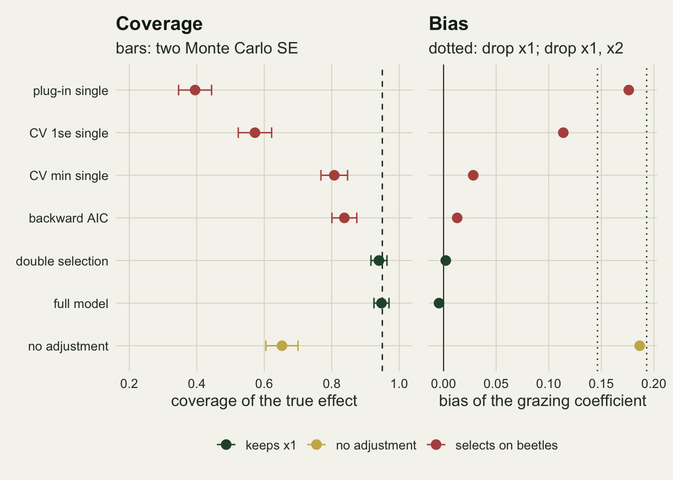
Drop pattern by drop pattern
Why the confounder goes is the mechanism Belloni and colleagues describe. With grazing in the model and unpenalised, a covariate is judged on what it adds to the prediction of beetles once grazing is known. Productivity is correlated with grazing, so part of its effect on beetles already comes through the grazing column. What it adds on its own is its effect times the square root of one minus its squared correlation with grazing, and that residual signal is what the penalty compares against its threshold. Backward AIC makes the same comparison with a gentler threshold: it drops a covariate when its t statistic is below 1.26 with all twenty covariates in the model and 1.37 once only the five that matter remain (the square root of two in large samples).
rho_x1 <- a_graze[1] / sqrt(v_graze)
signal_x1 <- b_main * sqrt(1 - rho_x1^2)
rho_x2 <- a_graze[2] / sqrt(v_graze)
signal_x2 <- b_rest[1] * sqrt(1 - rho_x2^2)
signal_x1_raw <- b_main * (1 - rho_x1^2)     # the same signal when the raw columns are standardised
thr_plugin <- plugin_level(n_sites, p_main) / (2 * n_sites)
thr_plugin01 <- plugin_level(n_sites, p_main, gamma = 0.1) / (2 * n_sites)
sel_arms <- c("plug-in single", "CV 1se single", "CV min single", "backward AIC")
pat_lev <- c("TRUETRUE", "FALSETRUE", "TRUEFALSE", "FALSEFALSE")
pat_lab <- c("x1 and x2 kept", "x1 dropped", "x2 dropped", "both dropped")
pm <- main_raw[main_raw$arm %in% sel_arms, ]
pm$pattern <- factor(pat_lab[match(pm$pat, pat_lev)], levels = pat_lab)
pat_tab <- do.call(rbind, lapply(split(pm, pm$pattern), function(d) data.frame(
  pattern = d$pattern[1], n = nrow(d), mean_est = mean(d$est), cover = mean(d$cover))))
pat_tab$closed <- c(0, bias_x1, bias_x2, bias_both)
pa <- function(k, what) pat_tab[k, what]
aic_pat <- table(factor(pm$pattern[pm$arm == "backward AIC"], levels = pat_lab)) / n_rep
On the standardised scale the residual signal of productivity is 0.244 and that of slope 0.233, while the plug-in threshold at this sample size is 0.359 times the residual standard deviation; the median penalty actually applied on the standardised scale, 0.359, shows that the residual standard deviation at the final pass is close to one. Both confounders sit below the line and are dropped nearly every time; moisture, altitude and pH, with no correlation to grazing, keep their full effects of 1.0, 0.8 and 0.5 and clear it. The comparison is approximate, since the lasso compares a covariate’s correlation with the current residual rather than its true coefficient, but it is enough to see that the outcome is largely decided by the constants, before any data are drawn. The choice of tail probability does not rescue it: with gamma = 0.1 instead of 0.1 / log(n) the threshold falls to 0.309, still above both residual signals. The cross-validated rules divide each column by its raw spread, which includes the part shared with grazing, so on their scale productivity’s signal is smaller again, b1 (1 - rho^2) = 0.198.
Pooling the four single-selection rules over the main cell and sorting the 1600 estimates by which confounders were kept, the mean estimate is -0.040 when both were kept, 0.110 when only productivity was dropped (closed form 0.146), 0.041 when only slope was dropped (0.100), and 0.195 when both were dropped (0.193). Coverage inside the four groups is 0.931, 0.725, 0.914 and 0.312. Only the group with both confounders dropped sits on its closed form, and it is the group the plug-in rule lands in for most surveys. The other three sit below theirs, because the choice is made on the same noise that sets the grazing estimate. A confounder is dropped in the surveys where its effect happens to look small, and it then passes that smaller apparent effect to grazing, not its true one. It is kept where its effect happens to look large, and because its estimate and the grazing estimate are negatively correlated (the two covariates overlap), a kept confounder comes with a grazing estimate pulled a little below zero. The closed form is the price of a fixed omission; a selected omission is conditioned on the noise. Backward AIC keeps both confounders in 0.650 of surveys and drops both in 0.098.
cl <- data.frame(pattern = factor(pat_lab, levels = pat_lab), closed = pat_tab$closed)
pm$arm_f <- factor(pm$arm, levels = sel_arms)
ggplot(pm, aes(est, pattern)) +
  geom_vline(xintercept = 0, colour = te_body, linetype = "dashed", linewidth = 0.5) +
  geom_jitter(aes(colour = arm_f), height = 0.25, width = 0, size = 0.9, alpha = 0.55) +
  geom_point(data = cl, aes(closed, pattern), shape = 124, size = 11, colour = te_rust) +
  scale_colour_manual(values = c(te_rust, te_gold, te_forest, "#8a8a7a"), name = NULL) +
  guides(colour = guide_legend(nrow = 2, override.aes = list(size = 2.5, alpha = 1))) +
  labs(x = "estimated grazing effect (truth 0)", y = NULL,
       title = "The omission sets the bias",
       subtitle = "dashed: true effect; red tick: omitted-variable bias for that pattern") +
  theme_datasheet() + theme(legend.position = "bottom")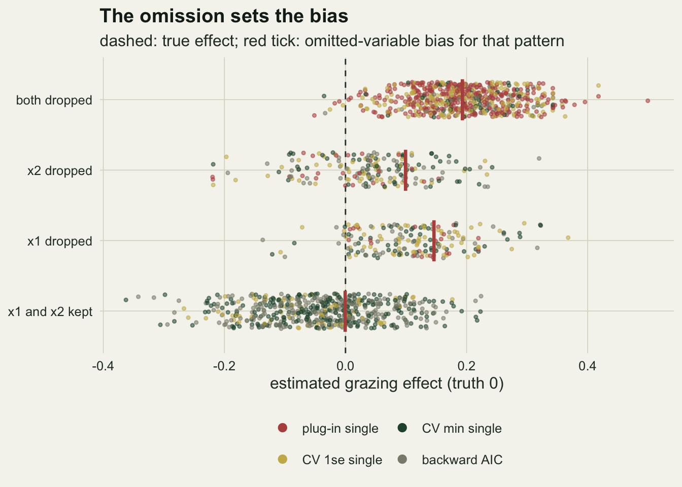
How strong a confounder has to be to vanish
The damage should be largest for a confounder strong enough to matter and weak enough to fall below the threshold. A weak one costs little when dropped; a strong one survives. The effect of productivity on beetles is varied with slope held at its value, and all other constants fixed. The cross-validated rules, which cost the most time, are run at three of the five values.
b1_grid <- c(0.15, 0.3, 0.45, 0.6, 0.9)
cv_grid <- c(0.15, 0.3, 0.6)
str_raw <- lapply(seq_along(b1_grid), function(k) {
  b1 <- b1_grid[k]
  if (b1 == b_main) main_raw else run_cell(2710 + k, n_sites, p_main, b1 = b1, do_cv = b1 %in% cv_grid)
})
str_tab <- do.call(rbind, Map(function(b1, m) cbind(b1 = b1, summarise_arms(m)), b1_grid, str_raw))
sa_at <- function(b1, arm, what) str_tab[str_tab$b1 == b1 & str_tab$arm == arm, what]
bias_x1_grid <- vapply(b1_grid, function(b) ovb(1, b), 0)
# the weakest-confounder cell, survey by survey
raw15 <- str_raw[[1]]
arm15 <- function(arm) raw15[raw15$arm == arm, ]
aic15 <- arm15("backward AIC")
share15 <- vapply(pat_lev, function(q) mean(aic15$pat == q), 0)
cov15 <- vapply(pat_lev, function(q) mean(aic15$cover[aic15$pat == q]), 0)
short15 <- 0.95 - mean(aic15$cover)                      # shortfall from nominal
short15_both <- share15[4] * (0.95 - cov15[4])           # the part owed to surveys dropping both
paired15 <- function(arm) { dd <- arm15("no adjustment")$cover - arm15(arm)$cover
  c(diff = mean(dd), se = sd(dd) / sqrt(length(dd))) }
d15_aic <- paired15("backward AIC"); d15_cvmin <- paired15("CV min single")
At the weakest confounder, 0.15, the plug-in single rule covers 0.650, the minimum-CV lasso 0.853 and backward AIC 0.858. At 0.6 backward AIC recovers to 0.920 and the minimum-CV lasso to 0.897, while the one-standard-error lasso is at 0.792 and the plug-in rule at 0.570, keeping productivity in 0.632 of surveys. At 0.9 the plug-in rule keeps it in 0.955 and covers 0.765. No adjustment gets steadily worse as the confounder strengthens, from 0.870 to 0.080; at the weakest confounder it covers as well as either the minimum-CV lasso or backward AIC (no adjustment minus each rule, paired over the same surveys: +0.018 and +0.013, with Monte Carlo standard errors 0.022 and 0.023), so selection there buys nothing over ignoring the covariates. Double selection stays between 0.927 and 0.963 over the whole range, and the full model is next to it throughout.
Slope never moves in this sweep, and it is a confounder too. At the weakest productivity effect backward AIC drops productivity in 0.573 of surveys and slope in 0.235. Its coverage falls 0.092 short of nominal, and 0.066 of that shortfall comes from the 0.175 of surveys that drop both, which cover 0.571. In the other three patterns coverage lies between 0.912 and 0.925.
line_arms <- c("plug-in single", "backward AIC", "double selection", "full model", "no adjustment")
pt_arms <- c("CV min single", "CV 1se single")
arm_col <- c("plug-in single" = te_rust, "backward AIC" = te_gold, "double selection" = te_forest,
             "full model" = te_ink, "no adjustment" = "#8a8a7a", "CV min single" = te_rust,
             "CV 1se single" = te_rust)
arm_shape <- c("CV min single" = 24, "CV 1se single" = 25)
sl <- str_tab[str_tab$arm %in% line_arms, ]; sp <- str_tab[str_tab$arm %in% pt_arms, ]
sl$arm <- factor(sl$arm, levels = line_arms); sp$arm <- factor(sp$arm, levels = pt_arms)
p_sc <- ggplot() +
  geom_hline(yintercept = 0.95, colour = te_body, linetype = "dashed", linewidth = 0.5) +
  geom_line(data = sl, aes(b1, cover, colour = arm), linewidth = 0.9) +
  geom_point(data = sl, aes(b1, cover, colour = arm), size = 2) +
  geom_point(data = sp, aes(b1, cover, shape = arm), colour = te_rust, fill = te_paper,
             size = 2.6, stroke = 0.9) +
  scale_colour_manual(values = arm_col[line_arms], name = NULL, limits = line_arms) +
  scale_shape_manual(values = arm_shape, name = NULL, limits = pt_arms) +
  scale_y_continuous(limits = c(0, 1)) +
  guides(colour = guide_legend(nrow = 3), shape = guide_legend(nrow = 2)) +
  labs(x = "effect of productivity on beetles", y = "coverage of the true effect",
       title = "Coverage") +
  theme_datasheet() + theme(legend.position = "bottom")
kl <- str_tab[str_tab$arm %in% c(line_arms[1:2], pt_arms), ]
kl$arm <- factor(kl$arm, levels = c(line_arms[1:2], pt_arms))
p_sk <- ggplot(kl, aes(b1, keep1)) +
  geom_line(data = kl[kl$arm %in% line_arms, ], aes(colour = arm), linewidth = 0.9) +
  geom_point(data = kl[kl$arm %in% line_arms, ], aes(colour = arm), size = 2) +
  geom_point(data = kl[kl$arm %in% pt_arms, ], aes(shape = arm), colour = te_rust,
             fill = te_paper, size = 2.6, stroke = 0.9) +
  scale_colour_manual(values = arm_col[line_arms], name = NULL, limits = line_arms) +
  scale_shape_manual(values = arm_shape, name = NULL, limits = pt_arms) +
  scale_y_continuous(limits = c(0, 1)) +
  guides(colour = guide_legend(nrow = 3), shape = guide_legend(nrow = 2)) +
  labs(x = "effect of productivity on beetles", y = "share of surveys keeping x1",
       title = "Is the confounder kept?") +
  theme_datasheet() + theme(legend.position = "bottom")
p_sc + p_sk + plot_layout(guides = "collect") +
  plot_annotation(theme = theme_datasheet() + theme(legend.position = "bottom"))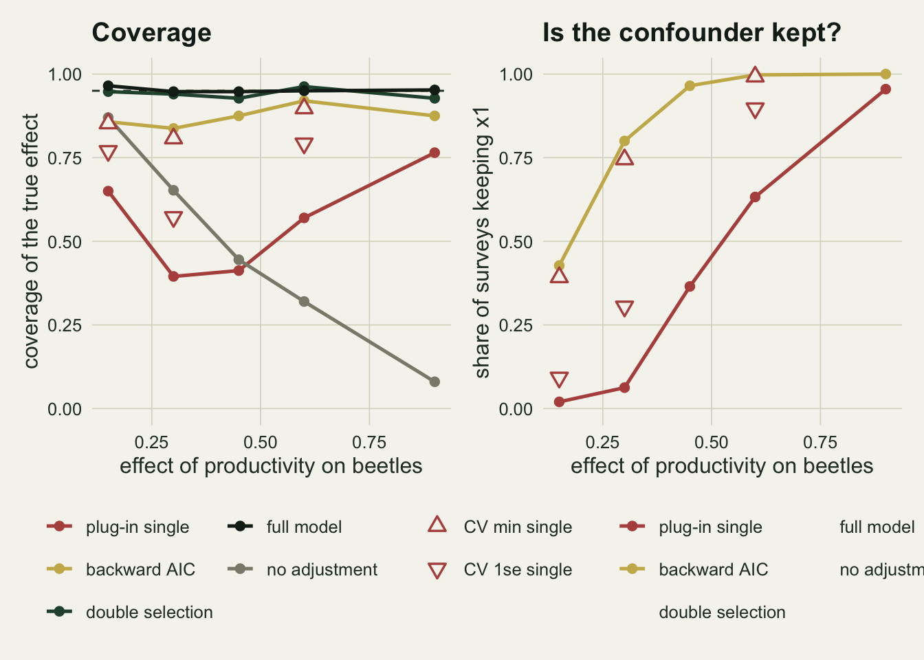
A real grazing effect changes nothing for single selection
It is tempting to rerun everything with a real grazing effect to check that the picture holds. For most of the rules there is nothing to check. Partialling grazing out of the beetle count removes any term proportional to grazing exactly, so the single-selection lasso sees the same residuals whatever the true effect is; backward AIC with grazing forced in compares residual sums of squares from which the grazing term has been fitted away; and the cross-validated rules refit grazing by least squares inside every fold. Each of these picks the same covariates on the same survey, and its estimate moves by exactly the true effect. Only the outcome half of double selection, which regresses beetles on the covariates without grazing, sees the change. Rerunning the main cell with the same seeds and a grazing effect of 0.5 shows it.
tau_alt <- 0.5
alt_raw <- run_cell(2701, n_sites, p_main, tau = tau_alt, do_cv = FALSE)
same_rows <- main_raw[main_raw$arm %in% c("plug-in single", "backward AIC", "full model", "no adjustment"), ]
alt_rows  <- alt_raw[alt_raw$arm %in% c("plug-in single", "backward AIC", "full model", "no adjustment"), ]
gap_replay <- max(abs((alt_rows$est - tau_alt) - same_rows$est))
alt_tab <- summarise_arms(alt_raw)
dbl_changed <- mean(alt_raw$pat[alt_raw$arm == "double selection"] != main_raw$pat[main_raw$arm == "double selection"])
For the plug-in single rule, backward AIC, the full model and no adjustment, the estimate minus the true effect is the same in the two runs up to floating-point rounding. Double selection keeps a different combination of the two confounders in 0.025 of surveys and covers 0.948 against 0.940 with no effect. A true effect of zero is therefore not a special case chosen to flatter the argument; the coverage of every single-selection rule is the same at any true effect.
Why use a lasso at all
At twenty covariates and a hundred pastures the full model is as good as double selection: it covers 0.948 against 0.940, and its standard deviation, 0.113, is barely above 0.106. If the design allows, the repair is not to select at all and to adjust for every pre-treatment covariate. The case for a lasso appears as the candidate list lengthens towards the number of sites.
The full model’s precision has a closed form here. Its estimate is unbiased, and its variance is the residual variance divided by the part of grazing not explained by the covariates, which is a chi-squared variable with n - p - 1 degrees of freedom; the expected inverse of that gives a standard deviation of 1 / sqrt(n - p - 3). An oracle that adjusts for exactly the five covariates that matter has 1 / sqrt(n - 8). Double selection can at best approach the oracle, and only if it finds the confounders.
p_grid <- c(20, 40, 60, 80)
wide_tab <- do.call(rbind, lapply(seq_along(p_grid), function(k) {
  pp <- p_grid[k]
  m <- if (pp == p_main) main_raw else run_cell(2720 + k, n_sites, pp, do_aic = FALSE, do_cv = pp == 60)
  cbind(p = pp, summarise_arms(m))
}))
wide_tab <- wide_tab[!(wide_tab$arm %in% c("backward AIC") & wide_tab$p > p_main), ]
wa <- function(pp, arm, what) wide_tab[wide_tab$p == pp & wide_tab$arm == arm, what]
sd_full_cf <- function(pp) 1 / sqrt(n_sites - pp - 3)
sd_oracle_cf <- 1 / sqrt(n_sites - 5 - 3)
At sixty covariates the full model’s standard deviation is 0.163 (closed form 0.164) and double selection’s 0.115, against the oracle’s 0.104. Both cover near nominal: 0.945 and 0.930. At eighty covariates the gap is wider, 0.252 (closed form 0.243) against 0.110. This is the answer to why an ecologist would use a lasso here: when the candidate list is a large fraction of the sample, double selection gives an estimate whose standard deviation is about 30 per cent smaller than the full model’s at sixty covariates, and its coverage stays near nominal.
The rules that select on the outcome alone get no such benefit. At sixty covariates the plug-in single rule covers 0.365, the minimum-CV lasso 0.615 with a bias of +0.084, and the one-standard-error lasso 0.450. Backward AIC is not run beyond twenty covariates; searching sixty or eighty terms one at a time would dominate the run time, and nothing in its mechanism changes with the width of the list.
cf <- data.frame(p = seq(20, 80, by = 1))
cf$full <- sd_full_cf(cf$p)
w_arms <- c("plug-in single", "double selection", "full model", "no adjustment")
wd <- wide_tab[wide_tab$arm %in% w_arms, ]; wd$arm <- factor(wd$arm, levels = w_arms)
p_wsd <- ggplot() +
  geom_line(data = cf, aes(p, full), colour = te_ink, linewidth = 0.8) +
  geom_hline(yintercept = sd_oracle_cf, colour = te_forest, linetype = "dashed", linewidth = 0.7) +
  geom_point(data = wd[wd$arm %in% c("double selection", "full model"), ],
             aes(p, sd, colour = arm), size = 2.8) +
  scale_colour_manual(values = arm_col[w_arms], name = NULL, limits = w_arms) +
  scale_y_continuous(limits = c(0, NA)) +
  labs(x = "candidate covariates", y = "SD of the grazing estimate", title = "Precision",
       subtitle = "solid: full model; dashed: oracle") +
  theme_datasheet() + theme(legend.position = "none")
p_wcov <- ggplot(wd, aes(p, cover, colour = arm)) +
  geom_hline(yintercept = 0.95, colour = te_body, linetype = "dashed", linewidth = 0.5) +
  geom_line(linewidth = 0.9) + geom_point(size = 2.2) +
  scale_colour_manual(values = arm_col[w_arms], name = NULL, limits = w_arms) +
  scale_y_continuous(limits = c(0, 1)) +
  guides(colour = guide_legend(nrow = 2)) +
  labs(x = "candidate covariates", y = "coverage of the true effect", title = "Coverage") +
  theme_datasheet() + theme(legend.position = "bottom")
p_wsd + p_wcov + plot_layout(guides = "collect") +
  plot_annotation(theme = theme_datasheet() + theme(legend.position = "bottom"))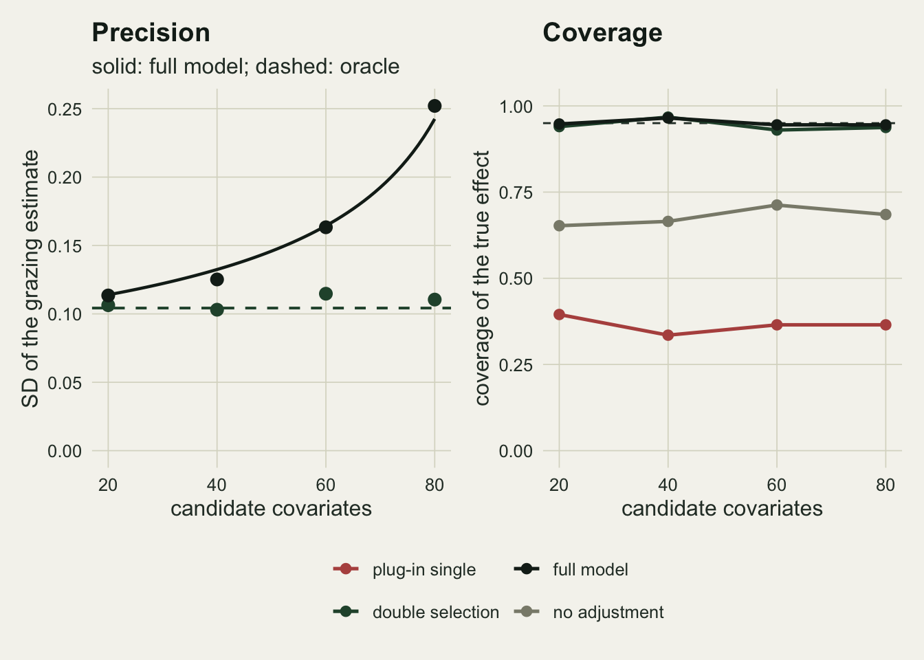
What to report
Say how the adjustment covariates were chosen, and report the list of candidates alongside the list that survived. If a confounder was on the candidate list and not in the final model, a reader needs to see that to judge the estimate.
When the number of candidates is small relative to the sample, do not select. Adjust for every pre-treatment covariate that could plausibly be a common cause, report that model, and treat the interval as an ordinary interval. At a hundred sites and twenty candidates the price here is a standard deviation of 0.113 against double selection’s 0.106, with no loss of coverage.
When the list is long enough that the full model’s interval is too wide, use double selection: a lasso of the outcome on the covariates, a lasso of the treatment on the covariates, and a least squares fit of the outcome on the treatment plus the union. Report both selected sets. Do not report an interval from a lasso or a stepwise search that chose covariates by the outcome alone, whichever penalty it used.
Double selection keeps anything that predicts the treatment, which is exactly why it works, and it will keep a mediator or a consequence of the treatment just as readily. The candidate pool must therefore contain only covariates fixed before the treatment was applied. The post on confounding and backdoor adjustment explains why a mediator in the adjustment set answers a different question; double selection has no way to tell a mediator from a confounder, so the pool has to be drawn up before the lasso sees it.
Honest limits
The design is kind to every rule. The covariates are independent normals, the effects are linear, the noise is Gaussian and homoscedastic, and the confounders are few and fixed. Correlated candidates would make the lasso’s choices between them unstable, as the site’s lasso and variable selection post shows, and would let a correlated stand-in for productivity carry part of its adjustment. Nothing here says how much that helps or hurts.
The coverage numbers belong to these effect sizes. With productivity’s effect on grazing at 0.8 and on beetles at 0.3 to 0.9, and slope held at 0.5 and 0.25, the single-selection rules fail at different strengths, and a different pair of confounders would move every rung of the ladder. The mechanism does not depend on the constants: any confounder whose residual signal falls below a rule’s threshold is dropped, and the omitted-variable formula gives the price.
The plug-in penalty is implemented here from its published form, with the tail probability set to 0.1 / log(n) and the loadings iterated from a five-covariate start; it is not checked against the authors’ own software, and other choices of constant move the threshold. The cross-validated rules standardise the raw columns, as cv.glmnet does when grazing is given a zero penalty factor. Standardising after grazing has been partialled out instead would raise productivity’s standardised signal by a factor 1 / sqrt(1 - rho^2) = 1.23 and keep it more often, so the two cross-validated rungs depend on that software convention as well as on the rule.
Double selection is the older, split-free member of a family of estimators. Chernozhukov and colleagues 2018 generalised it to double or debiased machine learning, with cross-fitting and flexible learners in both halves; the site’s post on doubly robust estimation points at the same family from the weighting side. None of that is covered here. And no selection rule, single or double, can adjust for a confounder that was never measured.
References
Belloni A, Chernozhukov V, Hansen C 2014 Review of Economic Studies 81(2):608-650 (10.1093/restud/rdt044)
Belloni A, Chernozhukov V, Hansen C 2014 Journal of Economic Perspectives 28(2):29-50 (10.1257/jep.28.2.29)
Leeb H, Potscher BM 2005 Econometric Theory 21(1):21-59 (10.1017/S0266466605050036)
Chernozhukov V, Chetverikov D, Demirer M, Duflo E, Hansen C, Newey W, Robins J 2018 Econometrics Journal 21(1):C1-C68 (10.1111/ectj.12097)
Tibshirani R 1996 Journal of the Royal Statistical Society B 58(1):267-288 (10.1111/j.2517-6161.1996.tb02080.x)