library(ggplot2)
library(patchwork)

te_paper  <- "#f5f4ee"
te_ink    <- "#16241d"
te_body   <- "#2c3a31"
te_forest <- "#275139"
te_rust   <- "#b5534e"
te_gold   <- "#c9b458"
te_line   <- "#dad9ca"

theme_datasheet <- function() {
  theme_minimal(base_size = 12) +
    theme(plot.background  = element_rect(fill = te_paper, colour = NA),
          panel.background = element_rect(fill = te_paper, colour = NA),
          panel.grid.major = element_line(colour = te_line, linewidth = 0.3),
          panel.grid.minor = element_blank(),
          text             = element_text(colour = te_body),
          plot.title       = element_text(colour = te_ink, face = "bold"),
          plot.subtitle    = element_text(colour = te_body),
          axis.text        = element_text(colour = te_body))
}Binning a time series invents a reverse cause
R
time series
Granger causality
temporal aggregation
simulation
ecology tutorial
Summing two time series into coarser bins makes a one-way driver look driven by its follower. A Granger test in R, with the repair: point samples, not sums.
This post is an R demonstration of a known consequence of temporal aggregation. Breitung and Swanson (2002) showed that when two time series are summed or averaged into ever wider bins, a lagged effect at the native step turns into same-time correlation between the bins, and Marcellino (1999) derived the aggregated process and studied what aggregation does to Granger causality. In practice, a cause that runs one way at the native time step can look as if it also runs the other way, and the standard lagged-regression test will often say so with a small p value. Nothing here is a new finding about that algebra. What the post adds is the size of the effect in a setting an ecologist would recognise, an arm that separates the effect from the loss of sample size that comes with binning, and a measured check of the repair (point samples), whose algebra is standard.
The setting is ordinary. A data logger records water temperature every day and a trap is emptied every day, and the question is whether the insect catch follows the temperature, whether the temperature follows the catch, or both. Put that way it sounds silly, because nobody expects a mayfly to warm a river, but the same data shape carries questions where both directions are plausible: does the predator track the prey or the prey respond to the predator, does grazing follow algal biomass or suppress it. The daily values are rarely analysed. They are summed into weekly or monthly totals, or averaged into monthly means, because that is how the data are archived, because the other series only exists at that step, or because a monthly figure looks cleaner. The directional test is then run on the bins.
The site already has the neighbouring warnings. Temporal autocorrelation and effective sample size shows two unrelated persistent series agreeing far more often than a naive test allows. Checking a time series model takes the same problem to the cross-correlation function and repairs it by prewhitening, with the time step fixed and trusted. Convergent cross mapping in ecology argues in prose that Granger’s test loses its footing in coupled nonlinear systems, for a different reason (the causal information has to be separable), and runs no Granger test. Checking an epidemic estimate spreads weekly case totals over days and measures what that costs one reproduction number: a bias in size, in one series, with no direction involved. None of them bins two series and asks a directional test to read the result. Here the time step itself is the choice under examination, and the answer is that prewhitening and extra lags only partly repair a wrong step, while the clean repair is to stop summing.
A driver, a follower and nothing flowing back
The generating process is the simplest one that has a known direction. The driver x is a first order autoregression with coefficient 0.7. The follower y has its own persistence of 0.5 and takes 0.6 of the driver’s value one step earlier. The two innovations are independent standard normals, and there is no term through which y can reach x. Every series is run for 300 steps before recording starts, so it begins effectively in its stationary state.
The test is the one Granger’s 1969 definition leads to and the one most packages call a Granger test: regress the candidate effect on its own lagged values, add the lagged values of the candidate cause, and compare the two nested least squares fits with an F test. The helper below does that with lm.fit instead of lm and anova, because it runs tens of thousands of times; the first check confirms that it returns the same p value as the textbook anova route.
a_x    <- 0.7    # persistence of the driver
a_y    <- 0.5    # persistence of the follower
b_xy   <- 0.6    # effect of the driver one step earlier on the follower
n_burn <- 300    # steps discarded before recording
alpha  <- 0.05

# columns are replicate series; the loop runs over time, not over series
gen_pair <- function(n_step, n_rep) {
  n_all <- n_step + n_burn
  x_m <- matrix(0, n_all, n_rep)
  y_m <- matrix(0, n_all, n_rep)
  e_x <- matrix(rnorm(n_all * n_rep), n_all)
  e_y <- matrix(rnorm(n_all * n_rep), n_all)
  for (i in 2:n_all) {
    x_m[i, ] <- a_x * x_m[i - 1, ] + e_x[i, ]
    y_m[i, ] <- a_y * y_m[i - 1, ] + b_xy * x_m[i - 1, ] + e_y[i, ]
  }
  keep <- (n_burn + 1):n_all
  list(x = x_m[keep, , drop = FALSE], y = y_m[keep, , drop = FALSE])
}

# block sums of k consecutive steps, one column per series
bin_sum <- function(v_m, k_bin) {
  n_b <- floor(nrow(v_m) / k_bin)
  if (k_bin == 1) return(v_m[seq_len(n_b), , drop = FALSE])
  rowsum(v_m[seq_len(n_b * k_bin), , drop = FALSE],
         rep(seq_len(n_b), each = k_bin), reorder = FALSE)
}

# the value at the last step of each bin: a point sample, not a total
take_every <- function(v_m, k_bin) v_m[seq(k_bin, nrow(v_m), by = k_bin), , drop = FALSE]

# nested F test: do p lags of `cause` improve an AR(p) model of `effect`?
lag_test <- function(effect, cause, p_lag) {
  idx  <- (p_lag + 1):length(effect)
  own  <- sapply(seq_len(p_lag), function(j) effect[idx - j])
  oth  <- sapply(seq_len(p_lag), function(j) cause[idx - j])
  x_0  <- cbind(1, own)
  x_1  <- cbind(x_0, oth)
  rss0 <- sum(lm.fit(x_0, effect[idx])$residuals^2)
  rss1 <- sum(lm.fit(x_1, effect[idx])$residuals^2)
  df_2 <- length(idx) - ncol(x_1)
  pf((rss0 - rss1) / p_lag / (rss1 / df_2), p_lag, df_2, lower.tail = FALSE)
}

# rejection rates over the columns: false direction (y -> x), true (x -> y)
rej_rate <- function(x_m, y_m, p_lag) {
  n_s <- ncol(x_m)
  c(false = mean(vapply(seq_len(n_s), function(r) lag_test(x_m[, r], y_m[, r], p_lag), 0) < alpha),
    true  = mean(vapply(seq_len(n_s), function(r) lag_test(y_m[, r], x_m[, r], p_lag), 0) < alpha))
}

set.seed(8101)
chk <- gen_pair(120, 20)
p_gap <- max(vapply(1:20, function(r) {
  xs <- chk$x[, r]; ys <- chk$y[, r]; n_c <- length(xs)
  m_0 <- lm(xs[3:n_c] ~ xs[2:(n_c - 1)] + xs[1:(n_c - 2)])
  m_1 <- lm(xs[3:n_c] ~ xs[2:(n_c - 1)] + xs[1:(n_c - 2)] + ys[2:(n_c - 1)] + ys[1:(n_c - 2)])
  abs(anova(m_0, m_1)$`Pr(>F)`[2] - lag_test(xs, ys, 2))
}, 0))

# the fine-step coefficient matrix and its powers (rows: x equation, y equation)
a_mat <- matrix(c(a_x, b_xy, 0, a_y), 2)
mat_pow <- function(m_in, k_bin) Reduce(`%*%`, replicate(k_bin, m_in, simplify = FALSE))
upper_max <- max(vapply(1:24, function(k_bin) abs(mat_pow(a_mat, k_bin)[1, 2]), 0))
lower_3   <- mat_pow(a_mat, 3)[2, 1]
lower_12  <- mat_pow(a_mat, 12)[2, 1]
On 20 test series the anova p value and the helper’s are identical: the two routes agree.
One more fact belongs here because the repair later rests on it. Taking every k-th value of this process gives another first order autoregression, whose coefficient matrix is the fine matrix raised to the power k. The entry that would carry an effect of y on x is zero in the fine matrix, and it stays zero in every power: across powers 1 to 24 its largest absolute value is 0. The effect of x on y survives: it is 0.6 at the fine step, grows slightly to 0.654 at every third step because the driver’s own persistence feeds it, and then shrinks to 0.0408 at every twelfth. That is the algebraic reason point samples keep the direction. Sums and means are not point samples, and the rest of the post is about what they do instead.
Summing into bins reverses the verdict
The first arm is the one a reader would produce. Six hundred daily values of each series are summed into bins of 1, 3, 6 and 12 steps, and the test is run in both directions with one lag and with three. Only its three-step cell has the 200 bins that every cell of the second arm has; its wider cells mix bin width with sample size, which is why the second arm, not this one, carries the profile across widths. The replication, a thousand series per cell, was fixed before anything ran.
n_fine <- 600
n_rep  <- 1000
k_set  <- c(1, 3, 6, 12)
mc_se  <- function(p_hat) sqrt(p_hat * (1 - p_hat) / n_rep)

set.seed(2511)
fine <- gen_pair(n_fine, n_rep)
arm_a <- do.call(rbind, lapply(k_set, function(k_bin) {
  xb <- bin_sum(fine$x, k_bin); yb <- bin_sum(fine$y, k_bin)
  r_1 <- rej_rate(xb, yb, 1); r_3 <- rej_rate(xb, yb, 3)
  data.frame(k = k_bin, n_bin = nrow(xb),
             f1 = r_1[["false"]], t1 = r_1[["true"]],
             f3 = r_3[["false"]], t3 = r_3[["true"]])
}))
cor_fine <- mean(vapply(1:n_rep, function(r) cor(fine$x[, r], fine$y[, r]), 0))
xb3 <- bin_sum(fine$x, 3); yb3 <- bin_sum(fine$y, 3)
cor_bin3 <- mean(vapply(1:n_rep, function(r) cor(xb3[, r], yb3[, r]), 0))
a_row <- function(k_bin) arm_a[arm_a$k == k_bin, ]
The bin widths leave 600, 200, 100, 50 bins to analyse. The Monte Carlo standard error of a rejection rate is 0.016 at worst, for a rate of one half, and 0.0069 at the nominal level.
At the native step the test behaves. The false direction, y causing x, is rejected in 0.048 of series against a nominal 0.05, and the true direction in 1.000. Sum the same series into three-step bins and the false direction is rejected in 0.475 of them (Monte Carlo standard error 0.016), while the true direction stays at 1.000. Nearly half of these series, analysed at a three-step resolution, would be reported as feedback: the driver responding to its follower, significantly, with the true direction significant too.
Three lags in each regression do not remove it. At three-step bins the false direction falls to 0.152, which is 3.0 times the nominal rate, and at six-step bins it is 0.141. Adding lags is the regression’s version of prewhitening, and it only partly helps, because in the binned data the follower’s past really does predict the driver’s next total; the test answers its own question correctly, and the error is reading that as a daily-scale cause.
The problem is where the lead went. At the fine step x leads y by one day. With three-day bins, two of every three one-day leads start and finish inside the same bin, so they show up as association between the two totals of the same bin: the average same-time correlation is 0.493 between the daily values and 0.656 between the three-day totals. The binned pair is no longer the first order autoregression that the test is built for; a moving sum of an autoregression is a mixed autoregressive moving average process, and its own lagged values no longer summarise its state. The follower’s last total carries information about how the driver moved inside the last bin, which the driver’s own coarse total has lost, and the test credits that information to the follower as a cause. Breitung and Swanson give the algebra for aggregated vector autoregressions in the limit of wide bins, where the lagged link turns into same-time correlation between the bins, and Marcellino derives the aggregated process for the wider autoregressive moving average class and treats causality among the properties that aggregation affects.
The six- and twelve-step cells need care. The false rate falls to 0.278 and 0.098 there, and the true direction falls to 0.369 at twelve-step bins, but the number of bins has fallen to 50 at the same time. From this arm alone there is no telling whether the artefact fades because the bins widen or because there are fewer of them.
Holding the number of bins fixed
The second arm answers that. Instead of cutting a fixed 600-step series into fewer and wider bins, it lengthens the fine series so that every cell has 200 bins to analyse. Only the width of the bin changes from column to column. A 24-step width is added, twice the widest bin of the first arm.
n_bin_fix <- 200
k_fix     <- c(1, 3, 6, 12, 24)

set.seed(6143)
arm_b <- do.call(rbind, lapply(k_fix, function(k_bin) {
  z_s <- gen_pair(n_bin_fix * k_bin, n_rep)
  xb <- bin_sum(z_s$x, k_bin); yb <- bin_sum(z_s$y, k_bin)
  xp <- take_every(z_s$x, k_bin); yp <- take_every(z_s$y, k_bin)
  r_1 <- rej_rate(xb, yb, 1); r_3 <- rej_rate(xb, yb, 3)
  r_p <- rej_rate(xp, yp, 1)
  r_m1 <- rej_rate(xp, yb, 1)   # driver point-sampled, follower summed
  r_m2 <- rej_rate(xb, yp, 1)   # driver summed, follower point-sampled
  data.frame(k = k_bin, n_bin = nrow(xb),
             f1 = r_1[["false"]], t1 = r_1[["true"]],
             f3 = r_3[["false"]], t3 = r_3[["true"]],
             pf = r_p[["false"]], pt = r_p[["true"]],
             m1f = r_m1[["false"]], m1t = r_m1[["true"]],
             m2f = r_m2[["false"]], m2t = r_m2[["true"]])
}))
b_row <- function(k_bin) arm_b[arm_b$k == k_bin, ]
pt_z  <- max(abs(arm_b$pf - alpha)) / sqrt(alpha * (1 - alpha) / n_rep)

# lag-one autocorrelation of the driver's bin totals, exact from the AR(1) autocovariance
bin_ac <- function(k_bin) {
  cov_ij <- function(i_s, j_s) outer(i_s, j_s, function(a, b) a_x^abs(a - b))
  sum(cov_ij(1:k_bin, (k_bin + 1):(2 * k_bin))) / sum(cov_ij(1:k_bin, 1:k_bin))
}
ac_bin3  <- bin_ac(3)
ac_bin24 <- bin_ac(24)
With 200 bins in every cell the false direction is rejected in 0.063, 0.510, 0.488 and 0.257 of series at widths 1, 3, 6 and 12, and the true direction in 1.000, 1.000, 1.000 and 0.923. At twelve-step bins the false direction fires in 0.257 of series (standard error 0.014), 5.1 times the nominal rate, while the test still finds the true direction in 0.923 of them. The collapse of the true direction to 0.369 in the first arm was the loss of bins, and so was part of the fade in the false direction, which is 0.257 here against 0.098 there. The artefact does not need the true signal to be failing; the two sit side by side at widths where a reader would trust the true direction.
At 24-step bins both rates finally drop, the false one to 0.125 and the true one to 0.366. That is a different mechanism from the sample-size fade: the correlation between successive bin totals of the driver, which is 0.495 at three-step bins, is only 0.065 at 24-step bins, so neither lagged term has much left to find, in either direction. This is the direction of the wide-bin limit Breitung and Swanson analyse, in which the lagged link gives way to same-time correlation between the bins. Three lags at fixed 200 bins give 0.165, 0.268 and 0.165 at widths 3, 6 and 12.
prof_long <- function(tab, panel) {
  rbind(data.frame(k = tab$k, rate = tab$f1, what = "false direction, 1 lag", panel = panel),
        data.frame(k = tab$k, rate = tab$f3, what = "false direction, 3 lags", panel = panel),
        data.frame(k = tab$k, rate = tab$t1, what = "true direction, 1 lag", panel = panel))
}
prof_plot <- function(dat, ttl, sub_t) {
  ggplot(dat, aes(k, rate, colour = what, shape = what)) +
    geom_hline(yintercept = alpha, linetype = "dashed", colour = te_body, linewidth = 0.5) +
    geom_line(linewidth = 0.9) +
    geom_point(size = 2.4) +
    scale_x_log10(breaks = k_fix) +
    scale_colour_manual(values = c(te_rust, te_gold, te_forest), name = NULL) +
    scale_shape_manual(values = c(16, 17, 15), name = NULL) +
    coord_cartesian(ylim = c(0, 1)) +
    labs(x = "bin width (fine steps)", y = "share of series rejected",
         title = ttl, subtitle = sub_t) +
    theme_datasheet()
}
p_left  <- prof_plot(prof_long(arm_a, "a"), "One 600-step series",
                     "bins fall from 600 to 50")
p_right <- prof_plot(prof_long(arm_b, "b"), "200 bins in every cell",
                     "only the width changes")
(p_left | p_right) + plot_layout(guides = "collect") +
  plot_annotation(theme = theme_datasheet()) &
  theme(legend.position = "bottom")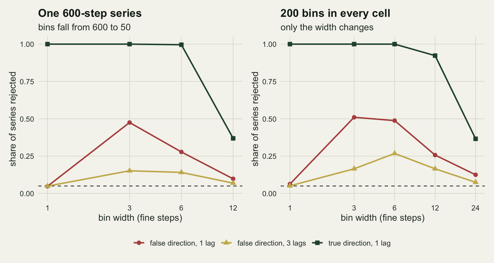
The prewhitened cross-correlation does not see through it
The time series check post reads lagged relationships from a prewhitened cross-correlation: fit a first order autoregression to the input series, filter both series with it, and look for lags whose correlation leaves the band of 1.96 over the square root of the series length. The same procedure is applied here to the false direction, with the follower as the input, on the daily values and on the three-day totals. The quantity recorded is the share of series in which each lag leaves the band.
pw_exceed <- function(inp, outp, lag_max = 3) {
  ph <- coef(arima(inp, order = c(1, 0, 0), method = "CSS"))[["ar1"]]
  i_w <- inp[-1] - ph * inp[-length(inp)]
  o_w <- outp[-1] - ph * outp[-length(outp)]
  cc  <- ccf(o_w, i_w, lag.max = lag_max, plot = FALSE)
  abs(as.numeric(cc$acf)) > 1.96 / sqrt(length(i_w))
}
# the same check without prewhitening, as a baseline
raw_exceed <- function(inp, outp, lag_max = 3) {
  cc <- ccf(outp, inp, lag.max = lag_max, plot = FALSE)
  abs(as.numeric(cc$acf)) > 1.96 / sqrt(length(inp))
}
lag_seq <- -3:3
ccf_tab <- do.call(rbind, lapply(c(1, 3), function(k_bin) {
  xb <- bin_sum(fine$x, k_bin); yb <- bin_sum(fine$y, k_bin)
  hit <- vapply(1:n_rep, function(r) pw_exceed(yb[, r], xb[, r]), logical(7))
  hit_raw <- vapply(1:n_rep, function(r) raw_exceed(yb[, r], xb[, r]), logical(7))
  data.frame(k = k_bin, lag = lag_seq, share = rowMeans(hit), share_raw = rowMeans(hit_raw))
}))
c_at   <- function(k_bin, h) ccf_tab$share[ccf_tab$k == k_bin & ccf_tab$lag == h]
c_raw  <- function(k_bin, h) ccf_tab$share_raw[ccf_tab$k == k_bin & ccf_tab$lag == h]
In ccf(o_w, i_w) a positive lag means the input, here the follower, leads. On the daily values the lag at which the follower leads the driver by one step leaves the band in 0.041 of series, the nominal 0.05 within sampling error, and the lag at which the driver leads by one step leaves it in 1.000. On the three-day totals the follower-leads lag leaves the band in 0.269 of series, against 0.871 for the same totals without prewhitening, and the same-bin lag, which was at 0.043 in the daily values, now leaves it in 1.000. (The daily bars at lags of minus two and minus three in the figure are the true lead again: the filter is fitted to the follower, so it does not fully whiten the driver, and the driver’s persistence spreads its real effect over several lags.) Prewhitening does the job it was built for, which is removing each series’ own persistence, and that removes most of the false lead. It cannot put back the ordering that summing destroyed, and a reader looking at the prewhitened plot of these totals would see a same-time spike in every series and, in 0.269 of them, a follower that appears to lead its driver.
ccf_tab$res <- factor(ifelse(ccf_tab$k == 1, "daily values", "three-step totals"),
                      levels = c("daily values", "three-step totals"))
ggplot(ccf_tab, aes(lag, share, fill = res)) +
  geom_col(position = position_dodge(width = 0.75), width = 0.7) +
  geom_hline(yintercept = alpha, linetype = "dashed", colour = te_body, linewidth = 0.5) +
  scale_fill_manual(values = c(te_forest, te_rust), name = NULL) +
  scale_x_continuous(breaks = lag_seq) +
  labs(x = "lag in bins (positive: follower leads driver)",
       y = "share of series outside the band",
       title = "Prewhitening keeps the reversed lead",
       subtitle = "dashed line: the nominal five per cent") +
  theme_datasheet() +
  theme(legend.position = "bottom")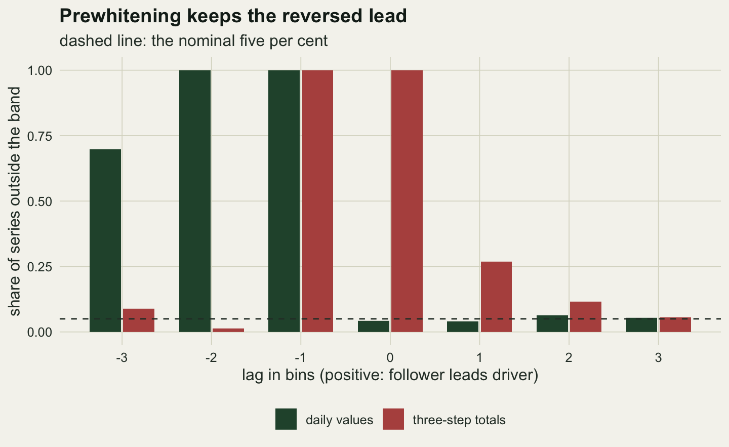
Point samples keep the direction, sums do not
Three checks locate the mechanism and give the repair. The first concerns means. Ecologists more often average a logger into a monthly mean than sum it, but a mean is a sum divided by a constant, and the F test with an intercept is unchanged when each series is multiplied by a constant. Means and sums therefore give the same p value to rounding, not just the same rate.
p_diff <- max(vapply(1:200, function(r)
  abs(lag_test(xb3[, r], yb3[, r], 1) - lag_test(xb3[, r] / 3, yb3[, r] / 3, 1)), 0))
Over 200 series at three-step bins the p values from sums and from means agree to 11 decimal places. Everything said about totals in this post applies unchanged to block means.
The second check replaces the bin total with the value at the last step of each bin, which is what a spot reading at the end of every month would give. The fixed-bin arm computed it on the same series. The false direction is rejected in 0.063, 0.039, 0.049, 0.041 and 0.059 of series at widths 1 to 24; the largest distance from the nominal level is 1.9 Monte Carlo standard errors. That is the matrix power argument from the first section, measured. (At width 1 the point sample and the total are the same series, so the first value is also the first cell of the fixed-bin profile.)
The third check mixes the two, because in field data the two series are often recorded differently: a logger can be read at a point, a trap catch is a total. With the driver point-sampled and the follower summed, the false direction is rejected in 0.044 of series at three-step bins and 0.063 at six-step bins. With the driver summed and the follower point-sampled it is 0.358 at three-step bins; at six-step bins that configuration falls back to 0.059, but its true direction has fallen to 0.288 as well. The reversal needs the driver to be aggregated. That follows from the setup: the driver’s point samples form a first order autoregression of their own, so given its last value nothing that happened earlier, the follower’s totals included, helps predict its next one.
That last sentence is also the condition on the repair. The matrix power argument needs the fine process to be a first order autoregression: its point samples are then first order again, and the driver’s last value carries everything its past knows. A driver with longer memory breaks that. The next chunk keeps the follower as before but gives the driver a second order autoregression with coefficients 1.2 and -0.5, a damped cycle, and runs the test with two lags on 200 point samples per series.
d_1 <- 1.2; d_2 <- -0.5   # a driver with second order memory

gen_ar2 <- function(n_step, n_rep) {
  n_all <- n_step + n_burn
  x_m <- matrix(0, n_all, n_rep)
  y_m <- matrix(0, n_all, n_rep)
  for (i in 3:n_all) {
    x_m[i, ] <- d_1 * x_m[i - 1, ] + d_2 * x_m[i - 2, ] + rnorm(n_rep)
    y_m[i, ] <- a_y * y_m[i - 1, ] + b_xy * x_m[i - 1, ] + rnorm(n_rep)
  }
  keep <- (n_burn + 1):n_all
  list(x = x_m[keep, , drop = FALSE], y = y_m[keep, , drop = FALSE])
}

set.seed(4409)
ar2_tab <- do.call(rbind, lapply(c(1, 3), function(k_bin) {
  z_s <- gen_ar2(n_bin_fix * k_bin, n_rep)
  r_2 <- rej_rate(take_every(z_s$x, k_bin), take_every(z_s$y, k_bin), 2)
  data.frame(k = k_bin, pf = r_2[["false"]], pt = r_2[["true"]])
}))
ar2_row <- function(k_bin) ar2_tab[ar2_tab$k == k_bin, ]
At the native step the two-lag test rejects the false direction in 0.044 of series. Point samples at every third step, with nothing summed, reject it in 0.358, while the true direction is found in 1.000. Every third value of a second order autoregression is not a second order autoregression, so the driver’s two last point samples no longer summarise its state and the follower’s past fills the gap, exactly as the totals did above. The point-sample repair is exact only for first order dynamics.
A nonlinear predator and its prey
The first question a time series econometrician would ask of all this is whether it is a property of linear Gaussian autoregressions being sold as ecology. The last arm swaps the generator for a nonlinear one at the fine step: a prey population with Ricker dynamics and lognormal environmental noise, and a predator whose growth depends on prey numbers through a saturating type II response and on its own density. The predator does not reduce prey numbers, so the true direction is still one way, prey to predator, with a one-step lag. That is the situation of a generalist predator that tracks one prey species without regulating it. The constants below were fixed before the arm was run and were not changed afterwards. Abundances are summed into bins and the test runs on the log of the bin totals, which is what would usually be done with them.
r_prey <- 0.3;  k_cap  <- 100;  s_prey <- 0.3
c_max  <- 1.5;  h_half <- 50;   m_die  <- 0.8
q_self <- 0.01; s_pred <- 0.2
k_pp   <- c(1, 3, 6, 12)

gen_pp <- function(n_step, n_rep) {
  n_all <- n_step + n_burn
  prey <- matrix(k_cap, n_all, n_rep)
  pred <- matrix(20, n_all, n_rep)
  for (i in 2:n_all) {
    prey[i, ] <- prey[i - 1, ] *
      exp(r_prey * (1 - prey[i - 1, ] / k_cap) + s_prey * rnorm(n_rep))
    pred[i, ] <- pred[i - 1, ] *
      exp(c_max * prey[i - 1, ] / (h_half + prey[i - 1, ]) - m_die -
          q_self * pred[i - 1, ] + s_pred * rnorm(n_rep))
  }
  keep <- (n_burn + 1):n_all
  list(x = prey[keep, , drop = FALSE], y = pred[keep, , drop = FALSE])
}

set.seed(7727)
pp_min <- Inf
arm_pp <- do.call(rbind, lapply(k_pp, function(k_bin) {
  z_s <- gen_pp(n_bin_fix * k_bin, n_rep)
  pp_min <<- min(pp_min, min(z_s$y))
  r_b <- rej_rate(log(bin_sum(z_s$x, k_bin)), log(bin_sum(z_s$y, k_bin)), 1)
  r_p <- rej_rate(log(take_every(z_s$x, k_bin)), log(take_every(z_s$y, k_bin)), 1)
  data.frame(k = k_bin, f1 = r_b[["false"]], t1 = r_b[["true"]],
             pf = r_p[["false"]], pt = r_p[["true"]])
}))
pp_row <- function(k_bin) arm_pp[arm_pp$k == k_bin, ]
With 200 bins in every cell, the false direction, predator causing prey, is rejected in 0.045 of series at the native step, then 0.221, 0.240 and 0.171 at bin widths 3, 6 and 12. The true direction is found in 1.000 of series at three-step bins. The nonlinear version is smaller than the linear one, but at every bin width above one it rejects at least 3.4 times as often as it should. Point samples again bring the false direction to the nominal rate: 0.037, 0.041 and 0.055 at the same three widths. The predator becomes very rare in some runs: the lowest value reached in any series was 0.00006. Abundances here are continuous, not counts, so that is a deep trough rather than an extinction, and the logs stay defined.
rep_long <- rbind(
  data.frame(k = arm_b$k, rate = arm_b$f1, how = "bin totals", model = "linear driver and follower"),
  data.frame(k = arm_b$k, rate = arm_b$pf, how = "point samples", model = "linear driver and follower"),
  data.frame(k = arm_pp$k, rate = arm_pp$f1, how = "bin totals", model = "prey and predator, nonlinear"),
  data.frame(k = arm_pp$k, rate = arm_pp$pf, how = "point samples", model = "prey and predator, nonlinear"))
ggplot(rep_long, aes(k, rate, colour = how, shape = how)) +
  geom_hline(yintercept = alpha, linetype = "dashed", colour = te_body, linewidth = 0.5) +
  geom_line(linewidth = 0.9) +
  geom_point(size = 2.4) +
  facet_wrap(~ model, scales = "free_x") +
  scale_x_log10(breaks = k_fix) +
  scale_colour_manual(values = c(te_rust, te_forest), name = NULL) +
  scale_shape_manual(values = c(16, 15), name = NULL) +
  coord_cartesian(ylim = c(0, 0.6)) +
  labs(x = "bin width (fine steps)", y = "false direction rejected",
       title = "Sums reverse the direction, point samples do not",
       subtitle = "dashed line: the nominal five per cent; 200 bins in every cell") +
  theme_datasheet() +
  theme(legend.position = "bottom", strip.text = element_text(colour = te_ink))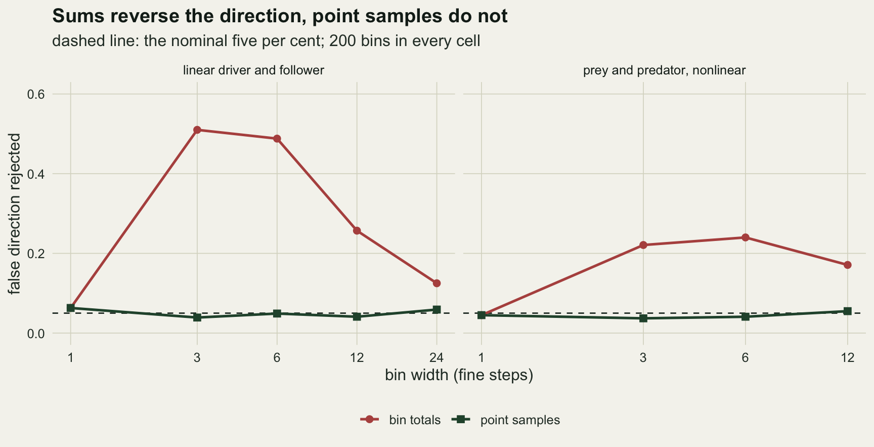
What point sampling costs
Point sampling keeps the test honest but discards most of the fine observations, and a population ecologist would want to know when that costs more than it saves. The last sweep holds the bin width at three and varies the length of the fine series from 60 to 960 steps, so the coarse series has 20 to 320 values. At each length it records the false-direction rate of the bin totals, which is the price of summing, and the true-direction rate of the point samples, which is the power the repair keeps. Both coarse versions have the same number of values, so the comparison is between two ways of using the same coarse clock.
n_fine_set <- c(60, 120, 240, 480, 960)
set.seed(3319)
len_tab <- do.call(rbind, lapply(n_fine_set, function(n_f) {
  z_s <- gen_pair(n_f, n_rep)
  r_f <- rej_rate(z_s$x, z_s$y, 1)
  r_b <- rej_rate(bin_sum(z_s$x, 3), bin_sum(z_s$y, 3), 1)
  r_p <- rej_rate(take_every(z_s$x, 3), take_every(z_s$y, 3), 1)
  data.frame(n_fine = n_f, n_coarse = n_f / 3,
             fine_t = r_f[["true"]], fine_f = r_f[["false"]],
             bin_f = r_b[["false"]], bin_t = r_b[["true"]],
             pt_f = r_p[["false"]], pt_t = r_p[["true"]])
}))
l_row <- function(n_f) len_tab[len_tab$n_fine == n_f, ]
At 20 coarse values the point samples find the true direction in only 0.541 of series, against 0.808 for the totals, while the totals’ false-direction rate is 0.114. At 40 values the point samples reach 0.865 and the totals’ false rate is 0.150. From 80 values upward the point samples find the true direction in at least 0.995 of series, while the totals’ false rate keeps climbing: 0.234, 0.400 and 0.630 at 80, 160 and 320 values. The false rate of summing grows with the length of the record, because the spurious feedback is a real feature of the aggregated process and a longer series estimates it more precisely. So the cost of point sampling is confined to very short series, which are exactly the ones where summing does least harm, and in long monitoring records there is no trade-off left to weigh. The fine series itself, analysed at its native step, found the true direction in 0.998 of series even at 60 steps, which is the better option whenever it exists.
len_long <- rbind(
  data.frame(n = len_tab$n_coarse, rate = len_tab$bin_f, what = "bin totals, false direction"),
  data.frame(n = len_tab$n_coarse, rate = len_tab$pt_t, what = "point samples, true direction"),
  data.frame(n = len_tab$n_coarse, rate = len_tab$pt_f, what = "point samples, false direction"))
ggplot(len_long, aes(n, rate, colour = what, shape = what)) +
  geom_hline(yintercept = alpha, linetype = "dashed", colour = te_body, linewidth = 0.5) +
  geom_line(linewidth = 0.9) +
  geom_point(size = 2.4) +
  scale_x_log10(breaks = len_tab$n_coarse) +
  scale_colour_manual(values = c(te_rust, te_gold, te_forest), name = NULL) +
  scale_shape_manual(values = c(16, 17, 15), name = NULL) +
  coord_cartesian(ylim = c(0, 1)) +
  labs(x = "values in the coarse series", y = "share of series rejected",
       title = "Summing gets worse as the record grows",
       subtitle = "three-step bins; dashed line: the nominal five per cent") +
  theme_datasheet() +
  theme(legend.position = "bottom") +
  guides(colour = guide_legend(nrow = 2), shape = guide_legend(nrow = 2))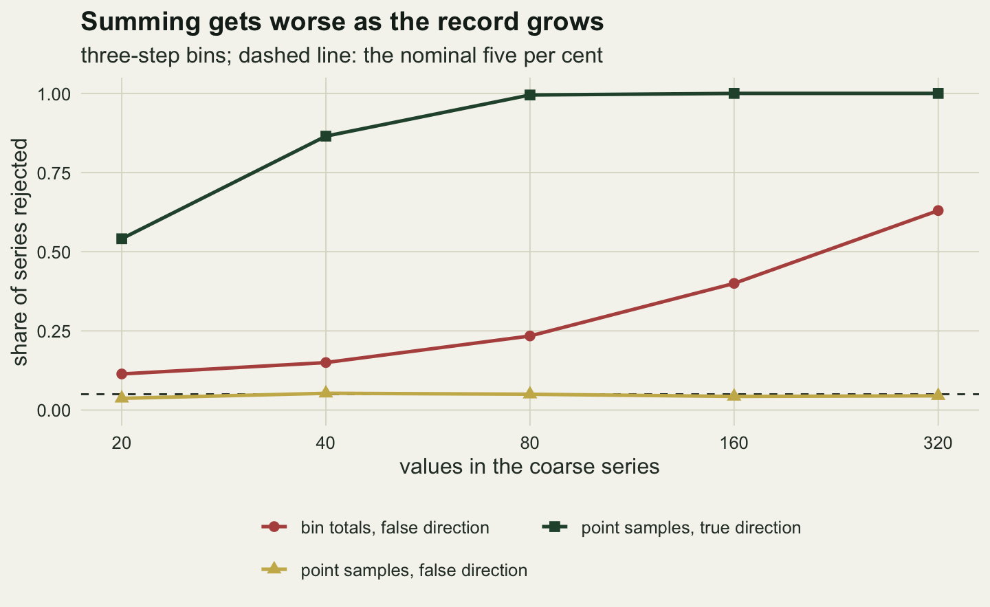
What to report
State the time step at which each series was recorded and the step at which it was analysed, and say whether each coarse value is a total, a mean or a point reading. A directional claim from binned data cannot be judged without those three facts, and in this post they decide whether a follower that has no effect on its driver is reported as causing it in 5 or in 48 per cent of series.
Run the test at the finest step both series share. If both were recorded daily, the daily test is valid here and loses nothing. A test of whether B drives A keeps its nominal rate when A, the candidate effect, is read at one point per bin, whether B was summed or point-sampled: with the driver point-sampled and the follower summed, the false direction came out at 0.044 and 0.063 at three- and six-step bins. That holds when A’s own dynamics are first order, as they were here. To test both directions, both series need a point reading, which is the point-sample arm above, where the true direction was found in 1.000 of series at three-step bins. When the candidate effect only exists as a total or a mean, a significant result cannot be told apart from aggregation, and it should be reported as association at that step, not as a direction.
Treat a significant reverse direction on binned data as a prompt, not a finding. A significant effect in both directions on binned data, together with a same-bin correlation well above the one at the native step (0.493 daily against 0.656 for three-day totals here), is the pattern aggregation produces. Adding lags cut the false rate here but left it 3.0 times the nominal level, and prewhitening the cross-correlation left the reversed lead visible, so neither should be offered as the fix.
Honest limits
The linear arms use one set of coefficients, a lag of exactly one fine step and independent innovations. A slower driver, a lag of several steps, or correlated shocks (a storm that raises both series on the same day) would be expected to change the size of the effect and possibly the width at which it peaks, and the post does not map that space. The magnitudes are measurements for this process; Breitung and Swanson’s algebra is the general statement, and it concerns the limit of wide bins, where the lagged link turns into same-time correlation, rather than the rejection rates shown here.
The nonlinear arm is one generator with constants chosen once. Its abundances are continuous and observed without error, so it says nothing about Poisson counts or detection. It shows that the reversal is not an artefact of linearity, not that its size carries over: the false rate there was 0.43 of the linear one at three-step bins, and a predator that regulated its prey would have a real reverse effect, which this post does not simulate.
Every test here is the nested least squares F test with a fixed lag order. Selecting the lag order by an information criterion, testing in a vector autoregression with a Wald statistic, or using a nonparametric causality measure could give different rates. The point-sample repair should carry over to them, because the matrix power argument is about the process and not about the test, as long as the process is a first order autoregression at the fine step. For a driver with longer memory, point samples give spurious feedback of their own (0.358 at three-step sampling with a two-lag test, in the second order case above), so the repair is exact only for first order dynamics.
The field ecologist’s question, how wide a bin can be before the artefact becomes negligible, has no clean answer from these runs. At 200 bins the false rate was still 0.257 at twelve steps, with the true direction almost always found, and at 24 steps it was still 0.125, by which width the true direction was found in only 0.366 of series. In these runs there was no width at which the true direction was reliably found and the false one was near nominal, other than the native step. Judging whether a bin is wide relative to the process requires knowing the lag and the persistence at the fine step, which is the thing the test was meant to find out.
Point sampling assumes the value at the sampled step is recorded without extra error. A spot reading of a noisy logger adds measurement error to the driver, which attenuates the true direction and may produce reverse effects of its own. That case belongs with the observation error problems in Checking a MAR(1) model and was not simulated here.
References
Breitung J, Swanson NR 2002 Journal of Time Series Analysis 23(6):651-665 (10.1111/1467-9892.00284)
Marcellino M 1999 Journal of Business and Economic Statistics 17(1):129-136 (10.1080/07350015.1999.10524802)
Granger CWJ 1969 Econometrica 37(3):424-438 (10.2307/1912791)