library(ggplot2)

te_paper  <- "#f5f4ee"
te_ink    <- "#16241d"
te_body   <- "#2c3a31"
te_forest <- "#275139"
te_rust   <- "#b5534e"
te_gold   <- "#c9b458"
te_line   <- "#dad9ca"

theme_datasheet <- function() {
  theme_minimal(base_size = 12) +
    theme(plot.background  = element_rect(fill = te_paper, colour = NA),
          panel.background = element_rect(fill = te_paper, colour = NA),
          panel.grid.major = element_line(colour = te_line, linewidth = 0.3),
          panel.grid.minor = element_blank(),
          text             = element_text(colour = te_body),
          plot.title       = element_text(colour = te_ink, face = "bold"),
          plot.subtitle    = element_text(colour = te_body),
          axis.text        = element_text(colour = te_body))
}Year trends in effect sizes and the SE covariate
R
meta-analysis
meta-regression
publication bias
simulation
ecology tutorial
A decline in effect size with publication year can be an artefact of growing samples. Measuring in R what the standard error covariate costs and which to use.
A review of nitrogen addition experiments and grassland species richness has eighty studies published between 1990 and 2023. Plot the standardised effects against publication year and the cloud tilts downwards: the early experiments reported large losses of species, the recent ones report smaller losses. A meta-regression on year gives a significant negative slope. The discussion section has two stories ready. One is ecological: deposition has fallen, or the recent experiments were run on sites that had already lost their sensitive species. The other is the decline effect, the pattern Jennions and Moller (2002) found across dozens of ecological and evolutionary meta-analyses, in which the first published effects are the largest and later ones shrink towards something smaller, and which Koricheva and Kulinskaya (2019) describe as temporal instability of the evidence base.
The mechanism that makes the second story possible is ordinary. Experiments get bigger over the decades, so early studies are small and imprecise. If small studies that found nothing were less likely to be published, the surviving early studies are the ones that overestimated, and year stands in for precision. The guidance ecologists now follow is to put both in one model: Nakagawa and colleagues (2022) set out a multilevel meta-regression with a precision covariate and the publication year as moderators, so that a year slope is read after the small-study effect has been removed. For standardised mean differences and log response ratios they recommend building that covariate from the effective sample size, the square root of (n1 + n2) / (n1 n2), rather than from the reported standard error, because the sampling variance of g contains g itself; Pustejovsky and Rodgers (2019) showed the false funnel asymmetry that the reported standard error produces in Egger’s test. Leimu and Koricheva (2004) brought cumulative meta-analysis, the running pooled estimate in publication order, into ecology as a tool for spotting such trends.
This post measures that recommendation rather than restating it. The decline effect, the year-plus-precision model and the advice to use the sample size version are known; what is measured here is how much power the precision covariate costs when the decline is real, and how much worse that cost is if a review uses the reported standard error instead of the recommended sample size version. For a standardised mean difference the two candidates are the square root of the reported sampling variance, which contains the effect size itself, and the square root of one over the effective sample size, which is built from sample sizes alone.
The neighbours on this site stop short of this. Checking for publication bias ties funnel asymmetry to study size through Egger’s regression on the standard error, and has no time axis. Inclusion criteria move the pooled effect writes a small year slope into its generating model and uses a year window as one of sixteen screening rules, but it never fits a year trend. Meta-regression with moderators shows a null moderator turning significant when the residual variance is left out, which is a different failure: its moderator is unrelated to precision. Collinearity and VIF in ecological regression supplies the mechanism for part of what follows, and one section below checks how much of the cost that mechanism accounts for.
A literature in which the studies grow
Each simulated study is a two-arm experiment published in a year drawn uniformly between 1990 and 2023. Its per arm sample size grows linearly from 8 in 1990 to 48 in 2023, with lognormal scatter around that line, so a study from the 1990s is usually small and one from the 2020s usually is not. The true effect is a mean of 0.2 at the middle of the window, plus a slope per decade that is zero or negative, plus a between-study standard deviation tau. Hedges g is computed from the sufficient statistics of two normal arms, and its sampling variance is the usual large sample formula, which contains g.
Publication is a filter on the sign and significance of the reported result. A study that is significantly positive at the two-sided 0.05 boundary is always published; every other study is published with probability w, which is 1 (no filter), 0.3 or 0.1. All of these constants were set before the first run.
yr_lo <- 1990; yr_hi <- 2023; yr_mid <- (yr_lo + yr_hi) / 2
n_start <- 8; n_end <- 48          # mean per arm sample size in 1990 and 2023
n_sdlog <- 0.3; n_floor <- 4       # lognormal scatter, smallest arm
mu_mid  <- 0.2                     # true mean effect at the middle year
z_crit  <- qnorm(0.975)

draw_synthesis <- function(k, tau, w_pub, slope) {
  out <- NULL
  while (is.null(out) || nrow(out) < k) {
    nb <- 6 * k
    year  <- runif(nb, yr_lo, yr_hi)
    n_mean <- n_start + (n_end - n_start) * (year - yr_lo) / (yr_hi - yr_lo)
    n_arm <- pmax(n_floor, round(n_mean * exp(rnorm(nb, 0, n_sdlog))))
    theta <- rnorm(nb, mu_mid + slope * (year - yr_mid) / 10, tau)
    dfree <- 2 * n_arm - 2
    mdiff <- rnorm(nb, theta, sqrt(2 / n_arm))
    s_pool <- sqrt(rchisq(nb, dfree) / dfree)
    g <- (1 - 3 / (4 * dfree - 1)) * mdiff / s_pool
    v <- 2 / n_arm + g^2 / (4 * n_arm)
    keep <- (g / sqrt(v) > z_crit) | (runif(nb) < w_pub)
    out <- rbind(out, cbind(year, n_arm, g, v)[keep, , drop = FALSE])
  }
  out[seq_len(k), ]
}
The meta-regression is a random effects model with a moment estimator of the residual tau-squared, the regression version of DerSimonian and Laird, written with matrices so it takes any number of moderators. The year slope is tested one-sided, because the claim under test is a decline. Three models are fitted to every synthesis: year alone; year and the standard error computed from the reported variance; and year and the square root of one over the effective sample size, which for two arms of n is the square root of two over n and does not involve g.
mreg_mom <- function(y, v, x_mat) {
  k <- length(y); p <- ncol(x_mat); w <- 1 / v
  xtw <- t(x_mat * w); a_inv <- solve(xtw %*% x_mat)
  b_fe <- a_inv %*% (xtw %*% y)
  q_res <- sum(w * (y - x_mat %*% b_fe)^2)
  tr_p <- sum(w) - sum(diag(a_inv %*% (t(x_mat * w^2) %*% x_mat)))
  tau2 <- max(0, (q_res - (k - p)) / tr_p)
  ws <- 1 / (v + tau2); xts <- t(x_mat * ws)
  v_b <- solve(xts %*% x_mat); b <- v_b %*% (xts %*% y)
  c(b = b[2], se = sqrt(v_b[2, 2]))
}

fit_three <- function(s, fitter = mreg_mom) {
  yc <- (s[, "year"] - yr_mid) / 10          # decades from the middle year
  se_g <- sqrt(s[, "v"]); se_n <- sqrt(2 / s[, "n_arm"])
  c(fitter(s[, "g"], s[, "v"], cbind(1, yc)),
    fitter(s[, "g"], s[, "v"], cbind(1, yc, se_g)),
    fitter(s[, "g"], s[, "v"], cbind(1, yc, se_n)),
    r_year_seg = cor(yc, se_g), r_year_sen = cor(yc, se_n),
    r_g_seg = cor(s[, "g"], se_g), r_seg_sen = cor(se_g, se_n))
}

set.seed(2016)
one_syn <- draw_synthesis(80, 0.2, 0.1, 0)
one_fit <- fit_three(one_syn)
one_fit
b se b se b se
-0.006030234 0.048793524 0.043348343 0.079972068 0.003552872 0.081675420
r_year_seg r_year_sen r_g_seg r_seg_sen
-0.798355280 -0.806783091 0.044915088 0.996427015 That is one filtered literature of 80 studies with no true change at all. The year-only slope is -0.006 per decade with a z of -0.12. Adding the g-based standard error moves it to +0.043 and adding the sample size version to +0.004. Year and the g-based standard error correlate at -0.80 in this synthesis, and the two standard errors correlate with each other at 0.996, so fitting both at once would ask the model to separate two near copies of one variable. One synthesis shows what the models do, not how often; the rest of the post counts.
The cumulative plot drifts down in both cases
The descriptive tool comes first because it is what most reviews show. Cumulative meta-analysis, as Leimu and Koricheva used it, orders the studies by publication year and re-pools after each addition. The chunk below computes it for three kinds of literature, one thousand syntheses of 80 studies each: no change and no filter, no change with a filter of 0.1, and a real decline of 0.1 per decade with no filter.
cum_dl <- function(y, v) {
  k <- length(y); w <- 1 / v
  s1 <- cumsum(w); s2 <- cumsum(w^2); sy <- cumsum(w * y); syy <- cumsum(w * y^2)
  tau2 <- pmax(0, (syy - sy^2 / s1 - (seq_len(k) - 1)) / (s1 - s2 / s1))
  ws <- 1 / outer(v, tau2, "+")             # row: study, column: step
  ws[row(ws) > col(ws)] <- 0                # study i enters at step i
  colSums(ws * y) / colSums(ws)
}

scen_cum <- data.frame(label = c("no change, all published", "no change, filter 0.1",
                                 "decline 0.1 per decade, all published"),
                       w = c(1, 0.1, 1), slope = c(0, 0, -0.1))
k_cum <- 80; n_cum <- 1000; first_step <- 5
set.seed(4131)
cum_runs <- lapply(seq_len(nrow(scen_cum)), function(i) {
  vapply(seq_len(n_cum), function(r) {
    s <- draw_synthesis(k_cum, 0.2, scen_cum$w[i], scen_cum$slope[i])
    s <- s[order(s[, "year"]), ]
    cum_dl(s[, "g"], s[, "v"])
  }, numeric(k_cum))
})
cum_tab <- do.call(rbind, lapply(seq_len(nrow(scen_cum)), function(i) {
  m <- cum_runs[[i]][first_step:k_cum, ]
  data.frame(step = first_step:k_cum, label = scen_cum$label[i],
             mid = apply(m, 1, median), lo = apply(m, 1, quantile, 0.1),
             hi = apply(m, 1, quantile, 0.9))
}))
cum_tab$label <- factor(cum_tab$label, levels = scen_cum$label)
cum_at <- function(i, step) cum_tab$mid[cum_tab$label == scen_cum$label[i] & cum_tab$step == step]
cum_drop <- vapply(seq_len(3), function(i) cum_at(i, 10) - cum_at(i, k_cum), 0)
After ten studies in publication order the median running estimate is 0.188 in the unfiltered literature with no change, 0.555 in the filtered one and 0.319 in the literature with a real decline. By the eightieth study they are 0.195, 0.480 and 0.168. Both leaning literatures drift down, by 0.075 in the filtered one and 0.151 in the one with a real decline, while the fair literature with no change moves by +0.007. The two drifts are not identical: the real decline keeps falling and crosses the mean of the middle year, while the filtered literature falls less and ends at more than twice the true mean. But that difference is only visible against a truth the reviewer does not have. On a real data set there is one curve, and a curve that drifts down fits either story. The cumulative plot shows that the pooled estimate moved and when; it has no way to say why, which is the answer to whether it is worth showing. It is a description of the literature, not a test of the system.
ggplot(cum_tab, aes(step, mid, colour = label, fill = label)) +
  geom_ribbon(aes(ymin = lo, ymax = hi), alpha = 0.12, colour = NA) +
  geom_line(linewidth = 1) +
  geom_hline(yintercept = mu_mid, colour = te_body, linetype = "dashed", linewidth = 0.5) +
  scale_colour_manual(values = c(te_ink, te_rust, te_gold), name = NULL) +
  scale_fill_manual(values = c(te_ink, te_rust, te_gold), name = NULL) +
  guides(colour = guide_legend(nrow = 3), fill = guide_legend(nrow = 3)) +
  labs(x = "studies included, in publication order", y = "running pooled Hedges g",
       title = "An artefact and a real decline both drift down",
       subtitle = "dashed line: the true mean at the middle year") +
  theme_datasheet() + theme(legend.position = "bottom")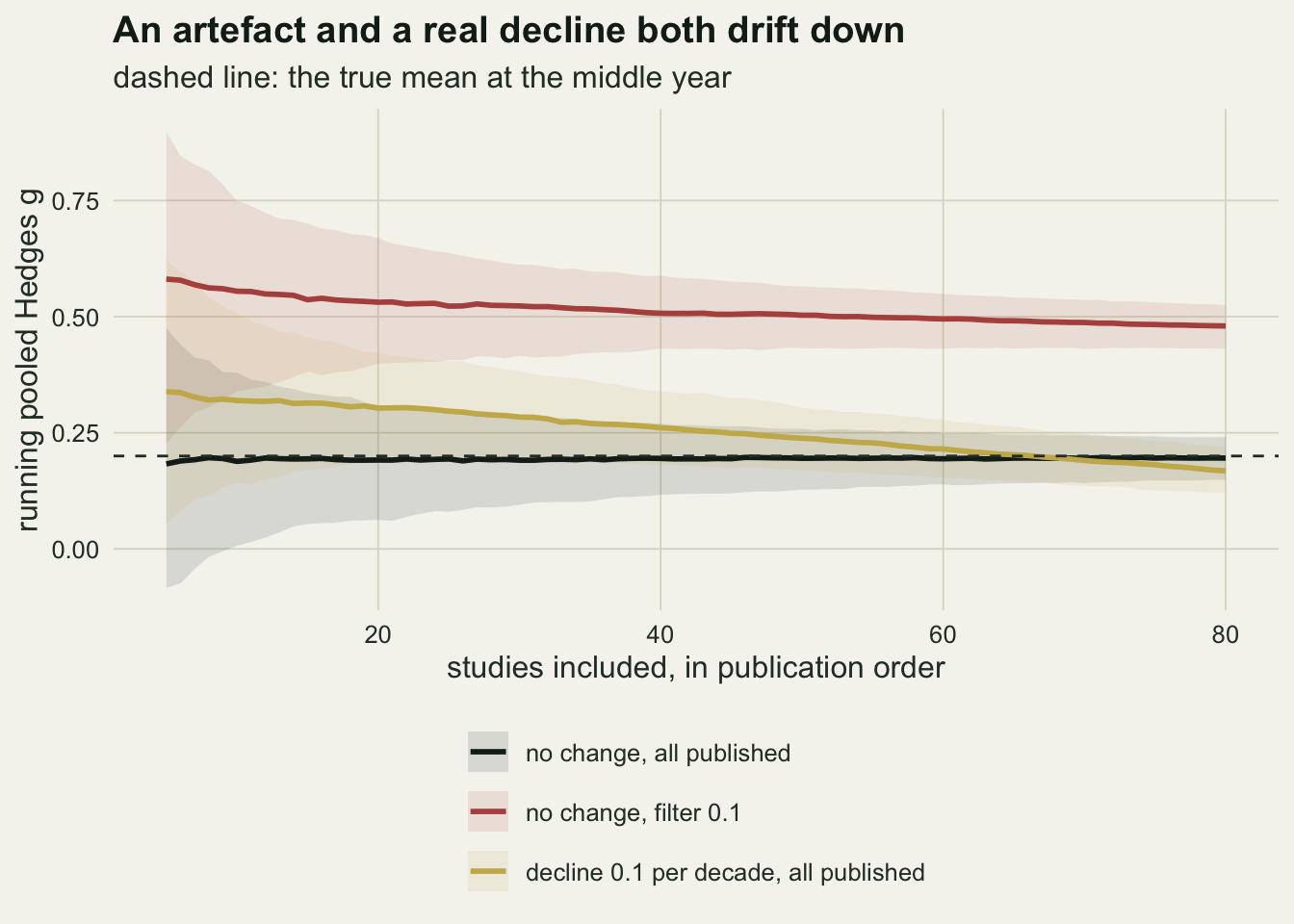
How often a decline appears that is not there
The main grid crosses three synthesis sizes, three publication probabilities and three true slopes, at a tau of 0.2, with one thousand syntheses per cell. That count was fixed before the grid was run; it puts the Monte Carlo standard error of a rate near the nominal 0.025 at about 0.005, and of a rate near one half at about 0.016.
k_grid <- c(40, 80, 150); w_grid <- c(1, 0.3, 0.1); slope_grid <- c(0, -0.05, -0.1)
n_rep <- 1000
model_lev <- c("year only", "year + SE from g", "year + SE from n")
summarise_cell <- function(m, slope) {
  z_dec <- function(j) mean(m[2 * j - 1, ] / m[2 * j, ] < -z_crit)
  data.frame(model = factor(model_lev, levels = model_lev),
             rate = vapply(1:3, z_dec, 0),
             slope_mean = vapply(1:3, function(j) mean(m[2 * j - 1, ]), 0),
             se_mean = vapply(1:3, function(j) mean(m[2 * j, ]), 0),
             r_year_seg = mean(m["r_year_seg", ]), r_year_sen = mean(m["r_year_sen", ]),
             r_g_seg = mean(m["r_g_seg", ]), r_seg_sen = mean(m["r_seg_sen", ]))
}
cells <- expand.grid(k = k_grid, w = w_grid, slope = slope_grid)
set.seed(7719)
grid_tab <- do.call(rbind, lapply(seq_len(nrow(cells)), function(i) {
  p <- cells[i, ]
  m <- vapply(seq_len(n_rep), function(r)
    fit_three(draw_synthesis(p$k, 0.2, p$w, p$slope)), numeric(10))
  rownames(m) <- names(fit_three(one_syn))
  cbind(p[rep(1, 3), ], summarise_cell(m, p$slope))
}))
grid_tab$mcse <- sqrt(grid_tab$rate * (1 - grid_tab$rate) / n_rep)
gt <- function(col, k, w, slope, j) grid_tab[[col]][grid_tab$k == k & grid_tab$w == w &
                                     grid_tab$slope == slope & grid_tab$model == model_lev[j]]
false_max_n <- max(grid_tab$rate[grid_tab$slope == 0 & grid_tab$model == model_lev[3]])
false_max_g <- max(grid_tab$rate[grid_tab$slope == 0 & grid_tab$model == model_lev[2]])
false_fair <- range(grid_tab$rate[grid_tab$slope == 0 & grid_tab$w == 1 & grid_tab$model == model_lev[1]])
With every study published, the year-only model declares a decline in between 0.020 and 0.026 of syntheses, against a nominal one-sided 0.025. With the filter at 0.1 the rate is 0.063 at 40 studies, 0.125 at 80 and 0.183 at 150, and it grows with the size of the synthesis because the artefact is a bias, not noise: the mean year-only slope in those cells is -0.026, -0.031 and -0.032 per decade, and more studies only shrink the standard error around it. At a publication probability of 0.3 there is nothing to see: the year-only rate is 0.026, 0.026 and 0.030 at the three sizes, and the mean slope at 80 studies is +0.002. In this design the artefact needs a strong filter.
So the false decline is real but modest. Even at the strongest filter and eighty studies it appears in about one synthesis in 8, 5.0 times the nominal rate, which is a reason for caution about a single year slope but not the main cost in this story. The main cost comes from the fix.
Both corrected models remove the false decline. The sample size covariate holds the false rate at or below 0.035 in every cell of the grid, a little above nominal at the strongest filter. The g-based covariate holds it at or below 0.012, under half the nominal rate even where there is no filter, which is the first sign that it does more than remove the artefact.
false_tab <- grid_tab[grid_tab$slope == 0, ]
false_tab$w_lab <- factor(sprintf("publication probability %.1f", false_tab$w),
                          levels = sprintf("publication probability %.1f", w_grid))
ggplot(false_tab, aes(k, rate, colour = model)) +
  geom_hline(yintercept = 0.025, colour = te_body, linetype = "dashed", linewidth = 0.5) +
  geom_errorbar(aes(ymin = rate - 2 * mcse, ymax = rate + 2 * mcse), width = 6, linewidth = 0.4) +
  geom_line(linewidth = 0.9) + geom_point(size = 2) +
  facet_wrap(~ w_lab) +
  scale_x_continuous(breaks = k_grid) +
  scale_colour_manual(values = c(te_forest, te_rust, te_gold), name = NULL) +
  labs(x = "studies in the synthesis", y = "false decline rate",
       title = "The artefact is a filter effect",
       subtitle = "dashed line: nominal one-sided 0.025; bars: two Monte Carlo SE") +
  theme_datasheet() + theme(legend.position = "bottom")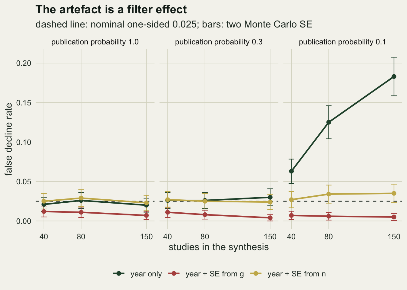
What the covariate costs when the decline is real
Now the same models on literatures where the true effect really falls by 0.1 per decade, which over the 33 year window takes it from 0.36 to 0.04. At 80 studies with the filter at 0.1, the year-only model detects it in 0.851 of syntheses. Adding the sample size covariate leaves 0.340, and adding the g-based standard error leaves 0.112. Without any filter the three are 0.611, 0.319 and 0.188, so the cost is paid whether or not there was anything to correct. At 150 studies and a filter of 0.1 the sample size model reaches 0.582 and the g-based model 0.189.
A decline of 0.05 per decade, half as steep, is mostly out of reach once the covariate is in. At 150 studies and no filter the year-only model detects it in 0.342 of syntheses, the sample size model in 0.188 and the g-based model in 0.077; with the filter at 0.1 the g-based model detects it in 0.029, barely above the nominal one-sided rate of 0.025 that a model with no decline in it should produce.
pw_tab <- grid_tab[grid_tab$slope < 0, ]
pw_tab <- pw_tab[pw_tab$w != 0.3, ]
pw_lev <- c("no filter, slope -0.05", "filter 0.1, slope -0.05",
            "no filter, slope -0.10", "filter 0.1, slope -0.10")
pw_tab$panel <- factor(sprintf("%s, slope %.2f", ifelse(pw_tab$w == 1, "no filter", "filter 0.1"),
                               pw_tab$slope), levels = pw_lev)
ggplot(pw_tab, aes(k, rate, colour = model)) +
  geom_errorbar(aes(ymin = rate - 2 * mcse, ymax = rate + 2 * mcse), width = 6, linewidth = 0.4) +
  geom_line(linewidth = 0.9) + geom_point(size = 2) +
  facet_wrap(~ panel, ncol = 2) +
  scale_x_continuous(breaks = k_grid) +
  scale_y_continuous(limits = c(0, 1)) +
  scale_colour_manual(values = c(te_forest, te_rust, te_gold), name = NULL) +
  labs(x = "studies in the synthesis", y = "share detecting a decline",
       title = "The correction costs most of the power",
       subtitle = "true slope per decade; bars: two Monte Carlo SE") +
  theme_datasheet() + theme(legend.position = "bottom")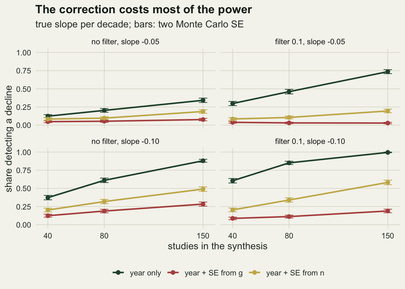
Which standard error goes into the model
The two corrected models differ by more than precision. Their mean year slopes in the no-change cells show it: at 80 studies and a filter of 0.1 the sample size model averages -0.002 per decade and the g-based model +0.047. With no filter at all the g-based model still averages +0.025. With a real decline of 0.1 and no filter, the sample size model recovers -0.099 and the g-based model -0.072.
The g-based model pushes the year slope upwards, towards no decline and past it, and the reason is in the variance formula. The sampling variance of g contains g squared, so a study that happened to overestimate also reports a larger standard error. That builds a positive association between the effect and the covariate inside every synthesis, with no selection at all, and a filter that keeps large positive effects strengthens it: the mean correlation between g and its own standard error is 0.04 without a filter and 0.19 with one, for the literature with no change. Part of that association is picked up by the coefficient of the standard error, and because year and the standard error are negatively correlated (-0.79 in that cell), the year slope moves the other way to compensate. The sample size covariate carries the same information about precision without the effect inside it.
sl_tab <- grid_tab[grid_tab$k == 80 & grid_tab$w != 0.3, ]
sl_tab$w_lab <- factor(sprintf("publication probability %.1f", sl_tab$w),
                       levels = sprintf("publication probability %.1f", c(1, 0.1)))
ggplot(sl_tab, aes(slope, slope_mean, colour = model)) +
  geom_abline(intercept = 0, slope = 1, colour = te_body, linetype = "dashed", linewidth = 0.5) +
  geom_line(linewidth = 0.9) + geom_point(size = 2.2) +
  facet_wrap(~ w_lab) +
  scale_x_continuous(breaks = slope_grid) +
  scale_colour_manual(values = c(te_forest, te_rust, te_gold), name = NULL) +
  labs(x = "true slope per decade", y = "mean estimated slope per decade",
       title = "The g-based standard error drags the slope up",
       subtitle = "dashed line: no bias; eighty studies per synthesis") +
  theme_datasheet() + theme(legend.position = "bottom")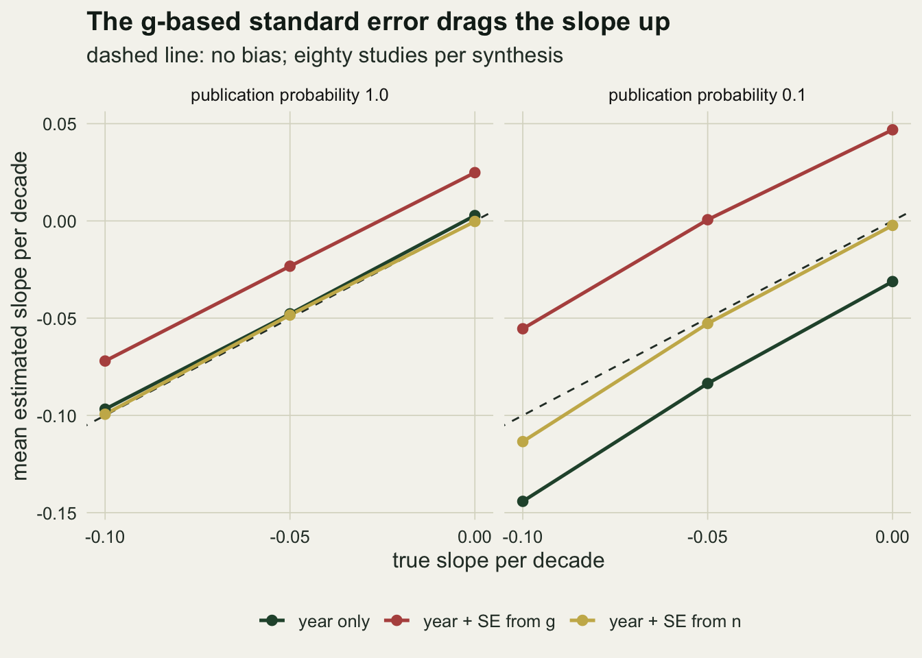
The moment estimator could be blamed for some of this. Nakagawa and colleagues fit by restricted maximum likelihood, so the headline cell is refitted that way below, on fresh syntheses, with tau-squared maximised by optimize.
mreg_reml <- function(y, v, x_mat) {
  neg_ll <- function(tau2) {
    ws <- 1 / (v + tau2); xts <- t(x_mat * ws); a_mat <- xts %*% x_mat
    b <- solve(a_mat, xts %*% y); r <- y - x_mat %*% b
    0.5 * (sum(log(v + tau2)) + determinant(a_mat)$modulus + sum(ws * r^2))
  }
  tau2 <- optimize(neg_ll, c(0, 2))$minimum
  ws <- 1 / (v + tau2); xts <- t(x_mat * ws)
  v_b <- solve(xts %*% x_mat); b <- v_b %*% (xts %*% y)
  c(b = b[2], se = sqrt(v_b[2, 2]))
}
n_reml <- 500
set.seed(5520)
reml_rates <- sapply(c(0, -0.1), function(sl) {
  m <- vapply(seq_len(n_reml), function(r) {
    s <- draw_synthesis(80, 0.2, 0.1, sl)
    c(fit_three(s)[1:6], fit_three(s, mreg_reml)[1:6])
  }, numeric(12))
  vapply(1:6, function(j) mean(m[2 * j - 1, ] / m[2 * j, ] < -z_crit), 0)
})
On 500 new syntheses of 80 studies with a filter of 0.1, the moment fits give false decline rates of 0.108, 0.004 and 0.024 (year only, g-based, sample size), and the REML fits 0.114, 0.004 and 0.032. With a real decline of 0.1 the detection rates are 0.870, 0.118 and 0.312 for the moment fits and 0.872, 0.120 and 0.318 for REML. The largest difference between the two methods is 0.008. The two methods were fitted to the same syntheses, so that is a difference between estimators rather than between random draws, and it is small against the gaps between the three models: the estimator of tau-squared is not what drives the cost.
More than a variance inflation factor
The natural reading of the power loss is collinearity: year and precision are correlated, the standard error of the year slope is inflated by the square root of the VIF, and power falls. The chunk below takes the headline cell, 80 studies with a filter of 0.1 and a true decline of 0.1 per decade, and rebuilds the corrected power in steps.
h_k <- 80; h_w <- 0.1; h_sl <- -0.1
p_year <- gt("rate", h_k, h_w, h_sl, 1)
r_yr <- gt("r_year_sen", h_k, h_w, h_sl, 1)
vif_cor <- 1 / (1 - r_yr^2)
se_year <- gt("se_mean", h_k, h_w, h_sl, 1)
vif_real <- (gt("se_mean", h_k, h_w, h_sl, 3) / se_year)^2
pred_power <- function(slope, se) pnorm(-slope / se - z_crit)
# step 1: deflate the year-only z by the square root of the VIF
p_vif <- pnorm((qnorm(p_year) + z_crit) / sqrt(vif_cor) - z_crit)
# step 2: the true slope instead of the inflated year-only slope
p_true <- pred_power(h_sl, se_year * sqrt(vif_cor))
# step 3: each corrected model's own mean slope and SE
p_own_n <- pred_power(gt("slope_mean", h_k, h_w, h_sl, 3), gt("se_mean", h_k, h_w, h_sl, 3))
p_own_g <- pred_power(gt("slope_mean", h_k, h_w, h_sl, 2), gt("se_mean", h_k, h_w, h_sl, 2))
vif_share_n <- (p_year - p_vif) / (p_year - gt("rate", h_k, h_w, h_sl, 3))
vif_share_g <- (p_year - p_vif) / (p_year - gt("rate", h_k, h_w, h_sl, 2))
vif_tab <- data.frame(
  step = c("year only, simulated", "VIF applied to the year-only z",
           "VIF applied, true slope", "SE from n: own slope and SE",
           "SE from n, simulated", "SE from g: own slope and SE", "SE from g, simulated"),
  power = c(p_year, p_vif, p_true, p_own_n, gt("rate", h_k, h_w, h_sl, 3),
            p_own_g, gt("rate", h_k, h_w, h_sl, 2)),
  kind = c("simulated", "predicted", "predicted", "predicted", "simulated", "predicted", "simulated"))
vif_tab$step <- factor(vif_tab$step, levels = rev(vif_tab$step))
The correlation between year and the sample size covariate in that cell is -0.80, a VIF of 2.76. The realised ratio of squared standard errors between the sample size model and the year-only model is 2.56, a little under the VIF because the weights are not equal, so the standard error inflates by close to what the VIF says. Applying that VIF to the year-only power of 0.851 predicts 0.440. The simulated power is 0.340 with the sample size covariate and 0.112 with the g-based one. The VIF step accounts for 81 per cent of the drop with the sample size covariate and 56 per cent with the g-based one.
The rest has two sources, and they are not the same for the two covariates. The first is that the year-only power was never the power to detect a decline of 0.1. Its mean slope was -0.144: the real decline plus the filter, which tilts harder when the true effects of recent studies are small, because more of those studies fall below significance. Deflating by the VIF but starting from the true slope gives 0.251, below even the simulated power of the sample size model. The sample size model’s own mean slope, -0.113, is still steeper than the truth, and with its own standard error it predicts 0.329, close to the simulated rate. So for this covariate the arithmetic is collinearity plus a residual tilt from the filter that the covariate does not fully remove.
The second source applies only to the g-based covariate: the upward drag on the slope from the previous section. Its mean slope is -0.055, about half the true decline, and with its own standard error that predicts 0.114. Collinearity explains why any covariate costs power here; the choice of covariate decides whether it also moves the estimate.
ggplot(vif_tab, aes(power, step, fill = kind)) +
  geom_col(width = 0.6, colour = te_paper, linewidth = 0.3) +
  geom_text(aes(label = sprintf("%.2f", power)), hjust = -0.2, colour = te_ink, size = 3.8) +
  scale_fill_manual(values = c(predicted = te_gold, simulated = te_forest), name = NULL) +
  scale_x_continuous(limits = c(0, 1.08), breaks = seq(0, 1, 0.25)) +
  labs(x = "power to detect the decline", y = NULL,
       title = "Collinearity is only part of the cost",
       subtitle = "gold: normal approximation, green: simulated") +
  theme_datasheet() + theme(legend.position = "bottom")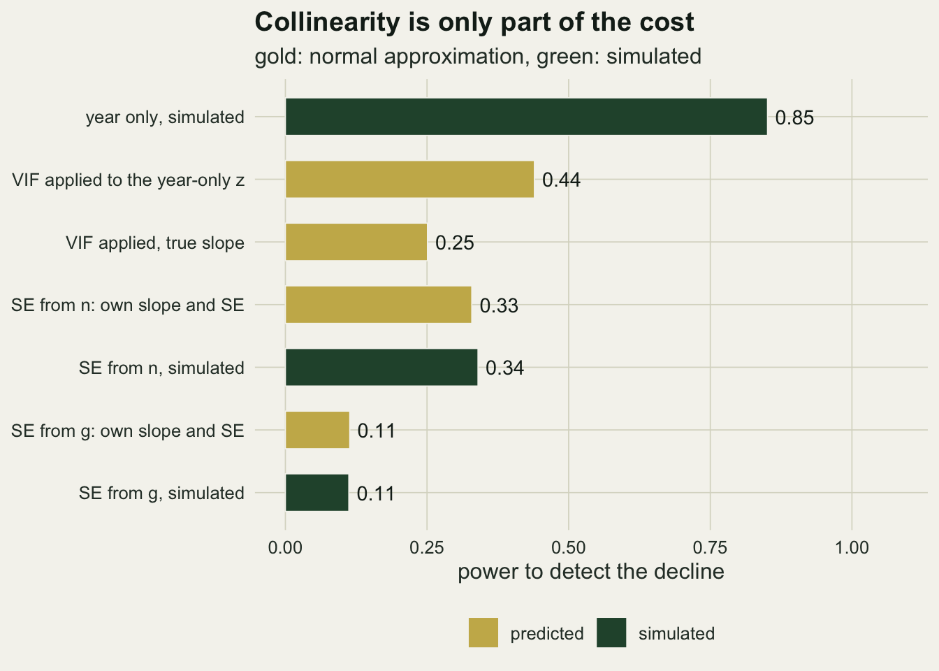
A smaller spread between studies
set.seed(8802)
tau_small <- 0.1
tau_tab <- do.call(rbind, lapply(c(1, 0.1), function(w) do.call(rbind, lapply(c(0, -0.1), function(sl) {
  m <- vapply(seq_len(n_rep), function(r)
    fit_three(draw_synthesis(80, tau_small, w, sl)), numeric(10))
  rownames(m) <- names(fit_three(one_syn))
  cbind(w = w, slope = sl, summarise_cell(m, sl))
}))))
tt <- function(w, sl, j) tau_tab$rate[tau_tab$w == w & tau_tab$slope == sl & tau_tab$model == model_lev[j]]
At a tau of 0.1 and 80 studies, the filter at 0.1 produces a false decline in 0.120 of year-only fits, 0.026 with the sample size covariate and 0.009 with the g-based one. A real decline of 0.1 is detected in 0.958, 0.497 and 0.240; without a filter in 0.773, 0.415 and 0.280. The ordering is the same as at a tau of 0.2. With the filter, the sample size model keeps 0.52 of the year-only power, and the g-based model keeps 0.48 of what the sample size model has left.
What to report
Report the year-only slope and the adjusted slope side by side, with their intervals, rather than only the model that reached significance. The pair carries the information: a slope that is steep alone and flat once precision is in the model is consistent with the artefact, and also with a real decline the adjusted model cannot see. In the headline cell the sample size model detected a real decline in 0.340 of syntheses, so a non-significant adjusted slope is weak evidence of no decline.
For a standardised mean difference, build the precision covariate from sample sizes, the square root of one over the effective sample size, and say so (the choice Nakagawa and colleagues recommend). The g-based standard error removed the false declines by pushing every year slope upwards, including real ones; its false decline rate stayed below the nominal level in every cell, which is the signature of a model that is biased towards the null rather than one that is calibrated. The two covariates correlate so closely (0.996 in the example synthesis) that fitting both is not a compromise; it is two copies of one variable with an effect-dependent difference between them.
Give the correlation between publication year and the precision covariate in the studies at hand. It is the number that says how much the adjusted model can separate, and a reader can turn it into a VIF. Near -0.80, as here, a decline of 0.1 per decade in a literature with no filter was detected by the sample size model in 0.490 of syntheses of 150 studies.
Evidence that a decline is real has to come from outside this regression. A trend in the driver itself, such as measured deposition or temperature at the study sites, can go in as a moderator in place of year. Studies that repeated one design at one site over years hold precision roughly fixed. A trend that persists among studies of similar size is harder to explain by the filter, although with a steep growth in sample size there are few such studies to compare. The cumulative plot adds none of this; it shows the drift both stories predict.
Honest limits
The filter is a single step: significant and positive studies are always published, the rest with one fixed probability. In this design the year slope needed a filter of 0.1 to appear, and a filter of 0.3 produced none. Real selection is graded, may depend on effect size as well as p value, and may itself change over the decades as journals changed their habits, which would create a year trend of its own that no precision covariate addresses.
Sample size grows linearly and deterministically with year, with the same lognormal scatter throughout. That fixes the correlation between year and precision near -0.80. A literature in which sample sizes grew less, or varied more within a year, would have a weaker correlation, a smaller VIF and a smaller cost; the numbers above are for one growth curve chosen before the runs, not an estimate of any real field.
Only Hedges g is simulated. The effect-dependent standard error is plainest for standardised mean differences and raw correlations, where the effect itself enters the variance formula. For a log response ratio the sampling variance uses the estimated means in the coefficients of variation, so it is also correlated with the ratio when arms are small, and Nakagawa and colleagues recommend the sample size covariate for it too; how large the drag is for a log response ratio was not measured here.
Every synthesis has one effect per study, and its sampling variance is the large sample formula with nothing else wrong with it. Nakagawa and colleagues fit a multilevel model because ecological syntheses have several effects per study. With several effects per study, year is constant within a study and its information comes only from between-study contrasts, which should make the cost larger rather than smaller, but that is an expectation, not a measurement. The fitting method was checked only in the headline cell, where REML and the moment estimator agreed, and the tests are z tests; a t-based adjustment of the standard errors would move every rate a little.
The true effect changes linearly with year. A step change, such as a single policy or a single event that shifted every later study, spreads over a linear year slope poorly, and a nonlinear trend in year would be confounded with a nonlinear relation to precision in ways this grid does not cover.
References
Jennions MD, Moller AP 2002 Proceedings of the Royal Society B 269(1486):43-48 (10.1098/rspb.2001.1832)
Leimu R, Koricheva J 2004 Proceedings of the Royal Society B 271(1551):1961-1966 (10.1098/rspb.2004.2828)
Koricheva J, Kulinskaya E 2019 Trends in Ecology and Evolution 34(10):895-902 (10.1016/j.tree.2019.05.006)
Nakagawa S, Lagisz M, Jennions MD, Koricheva J, Noble DWA, Parker TH, Sanchez-Tojar A, Yang Y, O’Dea RE 2022 Methods in Ecology and Evolution 13(1):4-21 (10.1111/2041-210X.13724)
Pustejovsky JE, Rodgers MA 2019 Research Synthesis Methods 10(1):57-71 (10.1002/jrsm.1332)