library(ggplot2)
library(patchwork)

te_paper  <- "#f5f4ee"
te_ink    <- "#16241d"
te_body   <- "#2c3a31"
te_forest <- "#275139"
te_rust   <- "#b5534e"
te_gold   <- "#c9b458"
te_line   <- "#dad9ca"

theme_datasheet <- function() {
  theme_minimal(base_size = 12) +
    theme(plot.background  = element_rect(fill = te_paper, colour = NA),
          panel.background = element_rect(fill = te_paper, colour = NA),
          panel.grid.major = element_line(colour = te_line, linewidth = 0.3),
          panel.grid.minor = element_blank(),
          text             = element_text(colour = te_body),
          plot.title       = element_text(colour = te_ink, face = "bold"),
          plot.subtitle    = element_text(colour = te_body),
          axis.text        = element_text(colour = te_body),
          strip.text       = element_text(colour = te_ink, face = "bold"))
}Vuong test for zero inflation, and what to use instead
R
count data
zero inflation
hypothesis testing
simulation
ecology tutorial
A Poisson is a zero-inflated Poisson with no inflation, so the Vuong test misfires. In R: its lost power, its false Poisson verdicts and the score test to use.
Fifty pitfall traps along a heathland transect, emptied after a week, and a ground beetle that turns up one or two at a time. Most traps hold a beetle or two, a good number hold none, and a few of the empty ones were found flooded or dug out by a badger, so they could not have caught anything. That is the textbook case for a zero-inflated Poisson: a mixture of a Poisson count and a separate process that produces structural zeros. The question the analysis starts with is whether the extra zero process is there at all, and the test many people reach for is the one pscl prints for them, the Vuong test of the zero-inflated fit against the plain Poisson.
The post on zero-inflated and hurdle models already tells you not to lean on that test. It cites Wilson (2015), who showed that a zero-inflated model and its plain counterpart do not meet the conditions Vuong (1989) set for comparing non-nested models, and it recommends information criteria instead. This post is a demonstration of Wilson’s result, not a claim to it. What it adds is the measurement behind that sentence: on counts with mild but real zero inflation the raw Vuong test rarely finds it, and the two corrected versions that pscl prints beside it certify the Poisson as significantly better, with certainty whenever the fitted zero-inflation probability sits on its boundary.
The boundary itself is not new on this site. The parametric bootstrap post tests Poisson against negative binomial, where the dispersion parameter of the null sits on the edge of its space, and shows that the naive chi-squared p-value is exactly twice the boundary-aware mixture one. That is a conservative test, fixed by halving. The Vuong test fails in a different direction: it is not a likelihood ratio test of nested models at all, and its corrected forms point at the wrong model.
A Poisson is a zero-inflated Poisson with no inflation
The zero-inflated Poisson gives a count of zero with probability pi + (1 - pi) exp(-lambda) and a count y > 0 with probability (1 - pi) times the Poisson probability of y. At pi = 0 it is the Poisson. The two models are nested, and the nesting point is on the edge of the parameter space, because a probability cannot be negative. Vuong’s test was built for the opposite situation, two models neither of which contains the other, and it compares them through the per-observation differences in log-likelihood, m_i. The statistic is the mean of m_i divided by its standard error; the AIC and BIC versions subtract a penalty for the extra parameter from the sum before dividing.
The code below fits both models by hand. The zero-inflated fit follows what pscl::zeroinfl does by default: BFGS on the log of lambda and the logit of pi, started from the Poisson mean and the logit of the observed share of zeros, with the same convergence tolerance. The one difference is that pscl supplies the analytic gradient, which this code leaves to the finite differences of optim. The Vuong statistics follow the source of pscl::vuong line by line, including the standard deviation with n - 1 in the denominator, the penalty of one parameter for the AIC version and log(n) / 2 for the BIC version, and a one-sided 5 per cent verdict in whichever direction the statistic points.
lam_true  <- 1.5                   # beetles per trap in a working trap
pi_set    <- c(0, 0.10, 0.20)      # share of traps that cannot catch
n_set     <- c(50, 100, 200)       # traps per survey
n_rep     <- 2000                  # surveys per cell, fixed before any rate was seen
alpha_lev <- 0.05
z_crit    <- qnorm(1 - alpha_lev)  # one-sided 5 per cent, as pscl prints it
bound_tol <- 1e-3                  # a fitted pi below this counts as on the bound

draw_survey <- function(n, p, lam = lam_true) {
  ifelse(runif(n) < p, 0L, rpois(n, lam))
}

# intercept-only ZIP: the likelihood needs only n0, n, sum(y) and sum(lgamma(y + 1))
zip_nll <- function(par, n0, n, sy, slg) {
  lam <- exp(par[1]); p <- plogis(par[2])
  -(n0 * log(p + (1 - p) * exp(-lam)) + (n - n0) * log1p(-p) +
      sy * log(lam) - (n - n0) * lam - slg)
}
fit_zip <- function(y) {
  n0 <- sum(y == 0); n <- length(y)
  start_par <- c(log(mean(y)), qlogis(min(max(n0 / n, 0.01), 0.99)))
  o <- optim(start_par, zip_nll, n0 = n0, n = n, sy = sum(y), slg = sum(lgamma(y + 1)),
             method = "BFGS",
             control = list(maxit = 10000, reltol = .Machine$double.eps^(1 / 1.6)))
  c(lam = exp(o$par[1]), pi = plogis(o$par[2]))
}
ll_zip_obs <- function(y, lam, p) {
  ifelse(y == 0, log(p + (1 - p) * exp(-lam)), log1p(-p) + dpois(y, lam, log = TRUE))
}

# the three statistics exactly as pscl::vuong computes them, ZIP as model 1
vuong_z <- function(m, k_diff = 1) {
  n <- length(m); s <- sd(m)
  c(raw = sum(m) / (s * sqrt(n)),
    aic = (sum(m) - k_diff) / (s * sqrt(n)),
    bic = (sum(m) - k_diff * log(n) / 2) / (s * sqrt(n)))
}

survey_tests <- function(y) {
  n <- length(y); ybar <- mean(y); n0 <- sum(y == 0)
  f <- fit_zip(y)
  m <- ll_zip_obs(y, f[["lam"]], f[["pi"]]) - dpois(y, ybar, log = TRUE)
  vz <- vuong_z(m)
  p0 <- exp(-ybar)
  u  <- n0 / p0 - n                                # score for pi at pi = 0
  info <- n * (1 - p0) / p0 - n * ybar             # its variance, lambda estimated
  c(n = n, n0 = n0, ybar = ybar, pi_hat = f[["pi"]],
    v_raw = vz[["raw"]], v_aic = vz[["aic"]], v_bic = vz[["bic"]],
    lr = max(0, 2 * sum(m)), z_score = u / sqrt(info),
    bound_num = f[["pi"]] < bound_tol, bound_cf = n0 / n <= p0)
}
The last two lines of survey_tests carry the closed form that the rest of the post leans on. With lambda at the Poisson estimate, the slope of the zero-inflated log-likelihood in pi at pi = 0 is u = n0 / exp(-ybar) - n, where n0 is the number of zero counts and ybar the mean count. If u is positive, a little zero inflation raises the likelihood and the estimate of pi moves inside; if u is zero or negative, the best pi is zero. So the estimate sits on the bound exactly when the observed share of zeros is no larger than exp(-ybar), the share a Poisson with the observed mean predicts. That is algebra, and the simulation below checks it against the numerical fit on every survey.
Two pitfall surveys and what pscl would print
Before any rates, one survey on each side of the bound. Surveys are drawn in a seeded sequence from the zero-inflated design with a tenth of the traps dead, and the first one that lands on the bound and the first one that does not are kept.
set.seed(611)
n_ex <- 50; p_ex <- 0.10
ex_bound <- NULL; ex_inner <- NULL; n_drawn <- 0
while (is.null(ex_bound) || is.null(ex_inner)) {
  y <- draw_survey(n_ex, p_ex); n_drawn <- n_drawn + 1
  tt <- survey_tests(y)
  if (tt[["bound_cf"]] && is.null(ex_bound)) { ex_bound <- tt; n_at_bound <- n_drawn }
  if (!tt[["bound_cf"]] && is.null(ex_inner)) { ex_inner <- tt; n_at_inner <- n_drawn }
}
ex_tab <- data.frame(survey = c("on the bound", "inside"),
  zeros = c(ex_bound[["n0"]], ex_inner[["n0"]]),
  poisson_zeros = n_ex * exp(-c(ex_bound[["ybar"]], ex_inner[["ybar"]])),
  pi_hat = c(ex_bound[["pi_hat"]], ex_inner[["pi_hat"]]),
  raw = c(ex_bound[["v_raw"]], ex_inner[["v_raw"]]),
  aic = c(ex_bound[["v_aic"]], ex_inner[["v_aic"]]),
  bic = c(ex_bound[["v_bic"]], ex_inner[["v_bic"]]),
  score_z = c(ex_bound[["z_score"]], ex_inner[["z_score"]]))
print(format(ex_tab, digits = 3), row.names = FALSE)
survey zeros poisson_zeros pi_hat raw aic bic score_z
on the bound 10 13.4 8.34e-06 -1.44 -13739.13 -26872.52 -1.489
inside 14 12.8 5.72e-02 0.24 -1.56 -3.27 0.519The first survey on the bound was draw 6 of the sequence and the first inside was draw 1. Both came from traps of which a tenth were dead.
The survey on the bound holds 10 empty traps where a Poisson with its mean predicts 13.4, so by the closed form the best pi is zero, and the numerical fit stops at pi = \(8.34 \times 10^{-6}\). Its raw Vuong statistic is -1.44, which says nothing. The AIC-corrected statistic is -13739 and the BIC-corrected one -26873: printed by pscl, those come with a p-value below any threshold and the line “model2 > model1”, the Poisson significantly better than the zero-inflated model on data that were generated with zero inflation.
The survey inside the bound has 14 empty traps against a Poisson expectation of 12.8, a fitted pi of 0.057, and Vuong statistics of 0.24, -1.56 and -3.27: the raw and AIC lines say nothing, and the BIC line, -3.27 against a critical value of -1.645, calls the Poisson significantly better even though the fit is off the bound. The score statistic in the last column, the test this post ends up recommending, is 0.52 against a one-sided critical value of 1.645.
Why the corrected statistics run to minus infinity
The size of that AIC statistic is not a quirk of one survey. At the bound the fitted lambda equals ybar and the zero-inflated fit is the Poisson plus a vanishing pi. To first order in the fitted pi, each difference m_i is pi-hat times (1{y_i = 0} / exp(-ybar) - 1) plus a lambda term that sums to zero over the survey. Two things follow.
The sum of m_i is pi-hat times u, and u is zero or negative on the bound, while the standard deviation of m_i is also proportional to pi-hat. The raw statistic is their ratio, so pi-hat cancels and the raw statistic stays finite and can never be positive on the bound. It cannot find zero inflation in a survey whose fit sits there.
The corrected statistics subtract a fixed penalty from the sum before dividing by a standard deviation that goes to zero with pi-hat. They go to minus infinity. In a numerical fit pi-hat stops at a tiny positive number, which is why the statistic in the worked example is large rather than infinite, and how large it gets depends on where the optimiser stopped. The verdict does not: on the bound, the corrected Vuong test declares the Poisson significantly better with probability one. That is algebra, and the main simulation checks it.
cells <- expand.grid(p = pi_set, n = n_set)
set.seed(3290)
sims <- do.call(rbind, lapply(seq_len(nrow(cells)), function(k) {
  r <- t(replicate(n_rep, survey_tests(draw_survey(cells$n[k], cells$p[k]))))
  data.frame(p = cells$p[k], r)
}))
sims$bound_num <- sims$bound_num == 1; sims$bound_cf <- sims$bound_cf == 1

agree_bound <- mean(sims$bound_num == sims$bound_cf)
n_disagree  <- sum(sims$bound_num != sims$bound_cf)
dis <- sims[sims$bound_num != sims$bound_cf, ]
dis_pi_max  <- if (nrow(dis)) max(dis$pi_hat) else NA_real_
dis_gap_max <- if (nrow(dis)) max(abs(dis$n0 / dis$n - exp(-dis$ybar))) else NA_real_
on_b <- sims$bound_cf
forced_aic <- mean(sims$v_aic[on_b] < -z_crit)
forced_bic <- mean(sims$v_bic[on_b] < -z_crit)
n_on_b     <- sum(on_b)
max_raw_b  <- max(sims$v_raw[on_b])
max_aic_b  <- max(sims$v_aic[on_b]); min_aic_b <- min(sims$v_aic[on_b])
forced_num <- mean(sims$v_aic[sims$bound_num] < -z_crit)
Across all 18000 simulated surveys the closed-form bound indicator and the numerical fit (pi-hat below 0.001) agree on 99.8 per cent of them; the 37 disagreements all have a fitted pi below \(9.2 \times 10^{-4}\) and an observed zero share within \(1.9 \times 10^{-4}\) of exp(-ybar), so they are surveys a hair from the boundary, where the numerical threshold and the exact condition fall on either side of a tiny fitted pi. On the 3882 surveys on the bound by the closed form, the AIC-corrected statistic returns a significant Poisson verdict in 1.000 of them and the BIC-corrected one in 1.000, with AIC statistics running from -5181611 to -87. The largest raw statistic among them is -0.009.
bd <- sims[sims$n == 50 & sims$p == 0.10, ]
min_inside <- min(bd$v_aic[!bd$bound_cf])
n_cell_b <- sum(bd$bound_cf); aic_rng_cell <- range(bd$v_aic[bd$bound_cf])
bound_slope <- unname(coef(lm(log(-v_aic) ~ log(pi_hat), data = bd[bd$bound_cf, ]))[2])
bd$state <- ifelse(bd$bound_cf, "on the bound", "inside")
squash <- function(v) asinh(v / 2)            # linear near zero, log far out
y_brk <- c(-1e4, -1e3, -100, -10, 0, 10)
bound_lab <- sprintf("%d surveys on the bound:\nstatistic from %.0f to %.0f", n_cell_b,
                     aic_rng_cell[1], aic_rng_cell[2])
ggplot(bd, aes(pi_hat, squash(v_aic), colour = state)) +
  geom_hline(yintercept = squash(c(-z_crit, z_crit)), colour = te_body,
             linetype = "dashed", linewidth = 0.5) +
  geom_point(size = 1, alpha = 0.45) +
  annotate("text", x = 2e-6, y = squash(-40), label = bound_lab, hjust = 0,
           colour = te_rust, size = 3.6) +
  annotate("text", x = 2e-6, y = squash(-z_crit) - 0.35, hjust = 0, size = 3.6,
           colour = te_body, label = "below: Poisson significantly better") +
  annotate("text", x = 2e-6, y = squash(z_crit) + 0.5, hjust = 0, size = 3.6,
           colour = te_body, label = "above: ZIP significantly better") +
  scale_x_log10(labels = scales::label_log()) +
  scale_y_continuous(breaks = squash(y_brk), labels = format(y_brk, big.mark = ",", trim = TRUE)) +
  scale_colour_manual(values = c(inside = te_forest, "on the bound" = te_rust),
                      name = NULL) +
  labs(x = "fitted zero-inflation probability (log scale)",
       y = "AIC-corrected Vuong statistic",
       title = "The corrected Vuong statistic at the boundary",
       subtitle = "50 traps, a tenth of them dead; dashed lines at the one-sided 5 per cent points") +
  theme_datasheet() + theme(legend.position = "bottom")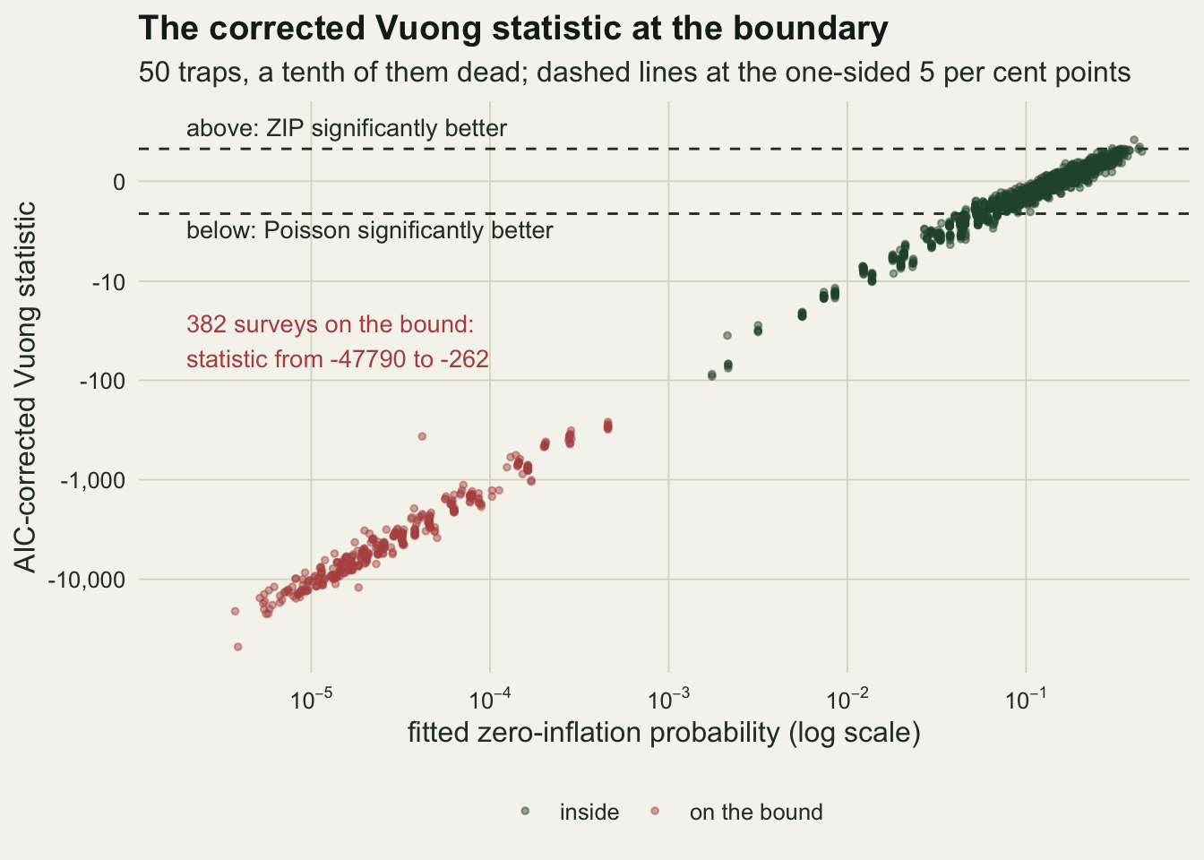
The picture has two populations. The fits on the bound sit at pi-hat values set by the optimiser’s stopping rule, far to the left, with statistics from -262 down to -47790. They fall along a straight line: regressing the log of the statistic’s magnitude on the log of pi-hat gives a slope of -0.98, so the statistic is close to proportional to 1 / pi-hat, as the algebra says. The fits inside spread across the plotted range, and 20 per cent of them also fall below the lower dashed line, down to -91.4. The most negative of them are fits just inside the bound, with a small pi-hat, where the same division by a small standard deviation is already at work; the boundary is where it becomes certain.
Nine designs, one direction at a time
The main grid crosses three truths (a Poisson, and zero inflation of a tenth and a fifth of the traps) with surveys of 50, 100 and 200 traps, 2000 surveys per cell. Every survey gets every procedure: the three Vuong statistics in both directions; the likelihood ratio test against a chi-squared on one degree of freedom, which ignores the boundary; the boundary-aware version, which uses the 50:50 mixture of a point mass at zero and a chi-squared on one degree of freedom (Self and Liang 1987), so its critical value is the 90 per cent point of the chi-squared; the van den Broek (1995) score test, one-sided in the excess-zero direction and two-sided; and plain AIC and BIC comparisons of the two fits.
rate_tab <- do.call(rbind, lapply(split(sims, list(sims$p, sims$n)), function(d) {
  nn <- d$n[1]
  data.frame(p = d$p[1], n = nn,
    raw_zip = mean(d$v_raw > z_crit),  raw_poi = mean(d$v_raw < -z_crit),
    aic_zip = mean(d$v_aic > z_crit),  aic_poi = mean(d$v_aic < -z_crit),
    bic_zip = mean(d$v_bic > z_crit),  bic_poi = mean(d$v_bic < -z_crit),
    lrt_chi1 = mean(d$lr > qchisq(1 - alpha_lev, 1)),
    lrt_bar  = mean(d$lr > qchisq(1 - 2 * alpha_lev, 1)),
    score1   = mean(d$z_score > z_crit),
    score2   = mean(d$z_score^2 > qchisq(1 - alpha_lev, 1)),
    ic_aic   = mean(d$lr > 2), ic_bic = mean(d$lr > log(nn)),
    bound    = mean(d$bound_cf), bound_num = mean(d$bound_num))
}))
rate_tab <- rate_tab[order(rate_tab$p, rate_tab$n), ]
rt <- function(col, p, n) rate_tab[[col]][rate_tab$p == p & rate_tab$n == n]
mcse <- function(r) sqrt(r * (1 - r) / n_rep)
print(format(rate_tab[, c("p", "n", "raw_zip", "score1", "lrt_bar", "lrt_chi1",
                          "ic_aic", "aic_poi", "bic_poi", "bound")], digits = 3),
      row.names = FALSE)
p n raw_zip score1 lrt_bar lrt_chi1 ic_aic aic_poi bic_poi bound
0.0 50 0.0005 0.0375 0.0370 0.0140 0.0620 0.7390 0.846 0.5405
0.0 100 0.0000 0.0445 0.0445 0.0245 0.0740 0.7120 0.855 0.4930
0.0 200 0.0005 0.0505 0.0490 0.0265 0.0785 0.7185 0.887 0.5185
0.1 50 0.0140 0.2140 0.2140 0.1390 0.2965 0.3555 0.520 0.1910
0.1 100 0.0325 0.3580 0.3580 0.2560 0.4460 0.2330 0.412 0.1000
0.1 200 0.0805 0.5810 0.5765 0.4470 0.6640 0.0930 0.261 0.0345
0.2 50 0.0505 0.4535 0.4535 0.3280 0.5615 0.1355 0.254 0.0495
0.2 100 0.1835 0.7405 0.7405 0.6385 0.8120 0.0360 0.113 0.0140
0.2 200 0.5445 0.9570 0.9565 0.9220 0.9750 0.0015 0.016 0.0000Start with 200 traps and a tenth of them dead. The raw Vuong test finds the zero inflation in 0.081 of the surveys. The one-sided score test finds it in 0.581 and the boundary likelihood ratio test in 0.577, 7.2 times the raw Vuong rate, with Monte Carlo standard errors of at most 0.011. In the same surveys the BIC-corrected Vuong test declares the Poisson significantly better 0.261 of the time and the AIC-corrected one 0.093.
At 50 traps it is worse. The raw test finds a tenth of dead traps in 0.014 of surveys, the boundary tests in 0.214 (likelihood ratio) and 0.214 (score), and the corrected Vuong tests call the Poisson significantly better in 0.355 (AIC) and 0.520 (BIC). With a fifth of the traps dead and 200 of them, the wrong verdict has almost gone (0.002 and 0.016) and the raw test reaches 0.544, still short of the 0.957 of the score test. The wrong-direction verdict lives where pi is small for the number of traps, which is where the question is hard and the answer matters.
proc_lev <- c("raw Vuong", "AIC-corrected Vuong", "BIC-corrected Vuong",
              "score test, one-sided", "boundary LRT", "plain AIC")
long_one <- function(col, proc, direction) {
  data.frame(p = rate_tab$p, n = rate_tab$n, rate = rate_tab[[col]],
             procedure = proc, direction = direction)
}
dir_lev <- c("prefers ZIP", "Poisson significantly better")
grid_df <- rbind(
  long_one("raw_zip", "raw Vuong", dir_lev[1]),
  long_one("score1", "score test, one-sided", dir_lev[1]),
  long_one("lrt_bar", "boundary LRT", dir_lev[1]),
  long_one("ic_aic", "plain AIC", dir_lev[1]),
  long_one("raw_poi", "raw Vuong", dir_lev[2]),
  long_one("aic_poi", "AIC-corrected Vuong", dir_lev[2]),
  long_one("bic_poi", "BIC-corrected Vuong", dir_lev[2]))
grid_df$procedure <- factor(grid_df$procedure, levels = proc_lev)
grid_df$direction <- factor(grid_df$direction, levels = dir_lev)
grid_df$truth <- factor(ifelse(grid_df$p == 0, "Poisson truth",
                               sprintf("ZIP, pi = %.2f", grid_df$p)),
                        levels = c("Poisson truth", sprintf("ZIP, pi = %.2f", pi_set[-1])))
grid_df$se2 <- 2 * mcse(grid_df$rate)
proc_col <- c(te_rust, te_gold, te_ink, te_forest, te_forest, te_body)
proc_lty <- c("solid", "solid", "solid", "solid", "dashed", "dotted")
proc_shp <- c(16, 17, 15, 16, 1, 4)
names(proc_col) <- names(proc_lty) <- names(proc_shp) <- proc_lev
ggplot(grid_df, aes(n, rate, colour = procedure, linetype = procedure, shape = procedure)) +
  geom_hline(yintercept = alpha_lev, colour = te_body, alpha = 0.5, linewidth = 0.5) +
  geom_errorbar(aes(ymin = rate - se2, ymax = rate + se2), width = 6,
                linewidth = 0.4, linetype = "solid") +
  geom_line(linewidth = 0.8) + geom_point(size = 2) +
  facet_grid(direction ~ truth) +
  scale_colour_manual(values = proc_col, name = NULL) +
  scale_linetype_manual(values = proc_lty, name = NULL) +
  scale_shape_manual(values = proc_shp, name = NULL) +
  scale_x_continuous(breaks = n_set) +
  scale_y_continuous(limits = c(0, 1)) +
  guides(colour = guide_legend(nrow = 2)) +
  labs(x = "traps per survey", y = "share of surveys",
       title = "Who finds the zeros, and who certifies the Poisson",
       subtitle = "grey line: 5 per cent") +
  theme_datasheet() + theme(legend.position = "bottom")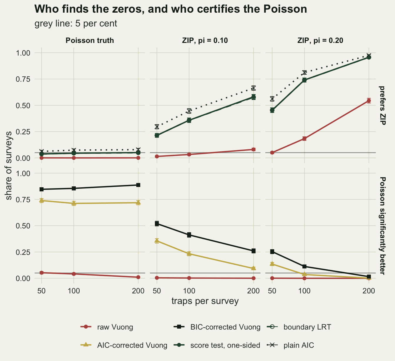
The Poisson column is the calibration check. There the boundary likelihood ratio test rejects 0.037, 0.044 and 0.049 of the time at 50, 100 and 200 traps, and the one-sided score test 0.037, 0.044 and 0.051. The raw Vuong test almost never prefers the zero-inflated model (at most 0.0005 of the surveys in a cell, 2 of the 6000 in all three), while the corrected versions call the true Poisson significantly better in 0.71 to 0.74 (AIC) and 0.85 to 0.89 (BIC) of surveys. The Poisson is the true model there, so the verdict is correct, but these are not the rates of a calibrated test. About half of these surveys sit on the bound, where the verdict is certain whatever the data say, and the corrected statistics add more Poisson verdicts from inside it; the rate mostly measures how often the fit touches the bound.
Four numbers that are arithmetic, not findings
Several rates in that table follow from the boundary before any simulation. Under a Poisson truth the score u is centred on zero and close to normal, so the fit lands on the bound in about half of all surveys. The naive likelihood ratio test uses the 95 per cent point of a chi-squared on one degree of freedom while half of the null mass of the statistic sits at zero, so its size tends to half the nominal 5 per cent. A plain AIC comparison prefers the zero-inflated model when the likelihood ratio statistic exceeds 2, so it is a likelihood ratio test at that threshold, with size one half of the chance that a chi-squared on one degree of freedom exceeds 2. Plain BIC is the same test with threshold log(n).
cf_bound <- 0.5
cf_chi1  <- 0.5 * alpha_lev
cf_aic   <- 0.5 * pchisq(2, 1, lower.tail = FALSE)
cf_bic   <- 0.5 * pchisq(log(n_set), 1, lower.tail = FALSE)
arith <- data.frame(n = n_set,
  bound_sim = rate_tab$bound[rate_tab$p == 0],
  chi1_sim  = rate_tab$lrt_chi1[rate_tab$p == 0],
  aic_sim   = rate_tab$ic_aic[rate_tab$p == 0],
  bic_sim   = rate_tab$ic_bic[rate_tab$p == 0], bic_cf = cf_bic)
print(format(arith, digits = 3), row.names = FALSE)
n bound_sim chi1_sim aic_sim bic_sim bic_cf
50 0.540 0.0140 0.0620 0.0135 0.0240
100 0.493 0.0245 0.0740 0.0135 0.0159
200 0.518 0.0265 0.0785 0.0110 0.0107The limits are 0.500 for the bound share, 0.025 for the naive test, 0.079 for plain AIC, and for plain BIC 0.024, 0.016 and 0.011 at 50, 100 and 200 traps. The simulated bound shares are 0.540, 0.493 and 0.518, the naive test’s sizes 0.014, 0.025 and 0.026, plain AIC 0.062, 0.074 and 0.079, and plain BIC 0.013, 0.013 and 0.011. The gaps are small-sample effects; the limits are asymptotic. None of these numbers is a result of this post. The result is in the three rates that do not have a closed form: the raw Vuong power, the wrong verdicts that happen inside the bound, and the gap to the boundary-aware tests.
The wrong verdict, split at the bound
The corrected Vuong rate of wrong verdicts is an average over two kinds of survey: the ones on the bound, where the verdict is certain, and the ones inside, where it is not. The split tells you how much of the problem is forced by the algebra.
split_tab <- do.call(rbind, lapply(split(sims[sims$p > 0, ], list(sims$p[sims$p > 0], sims$n[sims$p > 0])), function(d) {
  b <- d$bound_cf
  data.frame(p = d$p[1], n = d$n[1], n_bound = sum(b), n_inside = sum(!b),
    share_bound = mean(b),
    wrong_bound = if (any(b)) mean(d$v_aic[b] < -z_crit) else NA_real_,
    wrong_inside = mean(d$v_aic[!b] < -z_crit),
    wrong_all = mean(d$v_aic < -z_crit),
    forced_share = if (any(d$v_aic < -z_crit)) sum(b & d$v_aic < -z_crit) / sum(d$v_aic < -z_crit) else NA_real_)
}))
split_tab <- split_tab[order(split_tab$p, split_tab$n), ]
st <- function(col, p, n) split_tab[[col]][split_tab$p == p & split_tab$n == n]
print(format(split_tab, digits = 3), row.names = FALSE)
p n n_bound n_inside share_bound wrong_bound wrong_inside wrong_all
0.1 50 382 1618 0.1910 1 0.2033 0.3555
0.1 100 200 1800 0.1000 1 0.1478 0.2330
0.1 200 69 1931 0.0345 1 0.0606 0.0930
0.2 50 99 1901 0.0495 1 0.0905 0.1355
0.2 100 28 1972 0.0140 1 0.0223 0.0360
0.2 200 0 2000 0.0000 NA 0.0015 0.0015
forced_share
0.537
0.429
0.371
0.365
0.389
0.000At 200 traps with a tenth dead, 69 of the 2000 surveys land on the bound and every one of them gets the Poisson verdict; among the 1931 inside, the AIC-corrected test still calls the Poisson significantly better 0.061 of the time. Together that is the 0.093 above, and 37 per cent of those wrong verdicts are the forced ones on the bound. At 50 traps the bound holds 382 surveys, the inside rate is 0.203, and the forced share is 54 per cent.
So the algebra is not the whole story. Inside the bound the corrected statistic is finite, but its penalty is subtracted from a sum of per-trap differences that is small when the zero inflation is mild, and the ratio is often pushed below the lower critical value. The Vuong penalty was designed to be applied to two unrelated models of similar fit; here the models agree almost everywhere by construction.
sp_long <- rbind(
  data.frame(split_tab[, c("p", "n")], part = "forced on the bound",
             rate = split_tab$share_bound * ifelse(is.na(split_tab$wrong_bound), 0, split_tab$wrong_bound)),
  data.frame(split_tab[, c("p", "n")], part = "inside the bound",
             rate = (1 - split_tab$share_bound) * split_tab$wrong_inside))
sp_long$part <- factor(sp_long$part, levels = c("forced on the bound", "inside the bound"))
sp_long$truth <- sprintf("ZIP, pi = %.2f", sp_long$p)
ggplot(sp_long, aes(factor(n), rate, fill = part)) +
  geom_col(width = 0.6, colour = te_paper, linewidth = 0.3) +
  facet_wrap(~ truth) +
  scale_fill_manual(values = c(te_rust, te_gold), name = NULL) +
  labs(x = "traps per survey", y = "share of surveys: Poisson significantly better",
       title = "Where the wrong verdicts come from",
       subtitle = "AIC-corrected Vuong, one-sided 5 per cent") +
  theme_datasheet() + theme(legend.position = "bottom")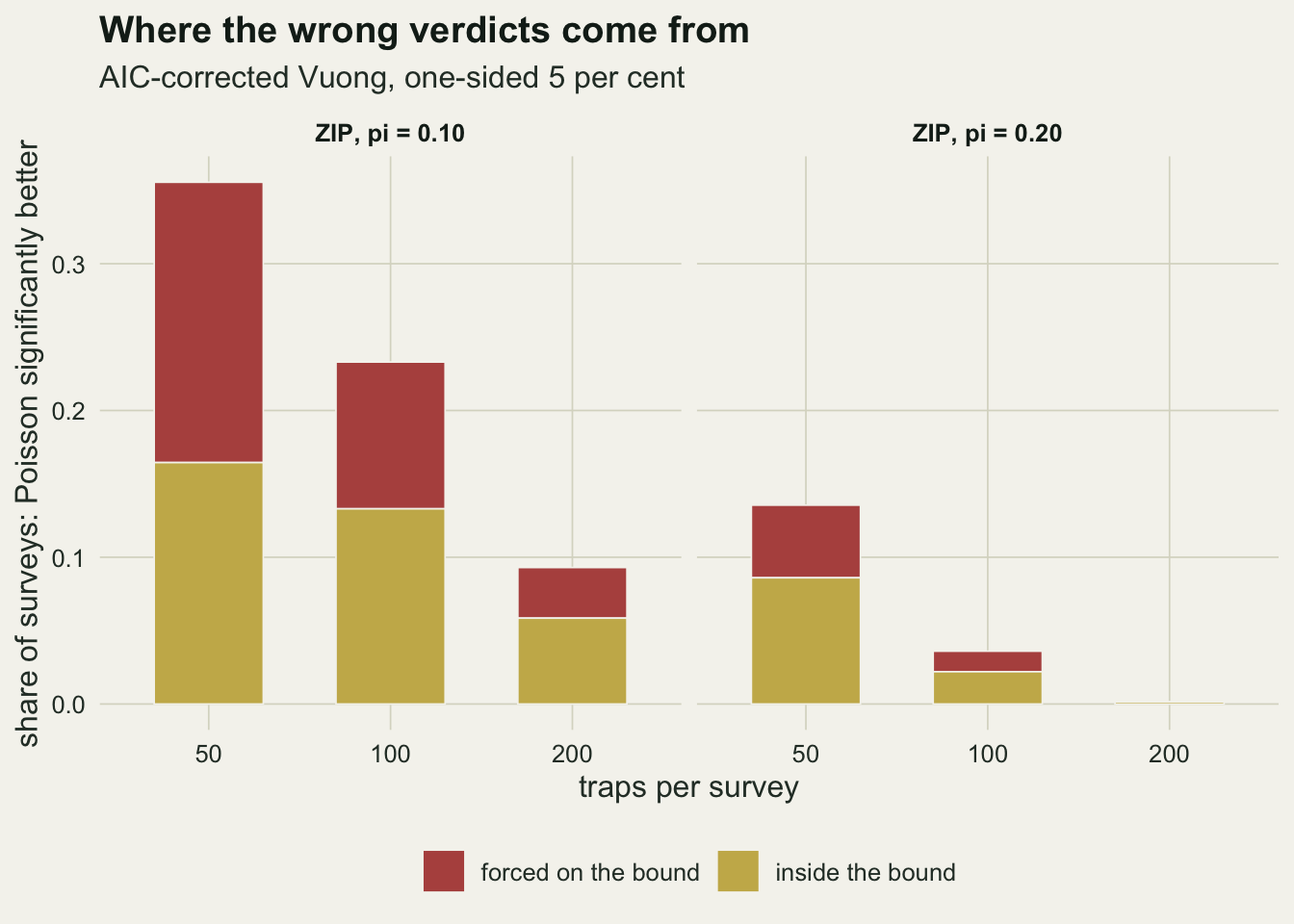
A covariate on the mean
Real zero-inflated models carry covariates, and a covariate changes the Poisson that the zeros are judged against: traps in wetter heath catch more beetles and should be empty less often. To check that nothing above depends on an intercept-only model, the same comparison is run with log lambda = b0 + 0.5 x for a standardised covariate x, the intercept set so that the average lambda stays at 1.5, a constant pi, and the zero-inflation part of the fit kept intercept-only, the model written y ~ x | 1 in pscl. The score test becomes van den Broek’s version with the covariate’s information removed from the variance, and the bound condition becomes the sign of the same score, which no longer has the simple zero-share form, so it is checked against the numerical fit.
b_slope <- 0.5
b_int   <- log(lam_true) - b_slope^2 / 2       # E[exp(b_slope * x)] = exp(b_slope^2 / 2)
n_rep_cov <- 500                              # fixed before any rate was seen
zipx_nll <- function(par, y, X, is0) {
  lam <- exp(drop(X %*% par[1:2])); p <- plogis(par[3])
  -sum(ifelse(is0, log(p + (1 - p) * exp(-lam)), log1p(-p) + dpois(y, lam, log = TRUE)))
}
survey_tests_x <- function(y, x) {
  n <- length(y); X <- cbind(1, x); is0 <- y == 0
  gp <- glm.fit(X, y, family = poisson()); mu <- gp$fitted.values
  start_par <- c(gp$coefficients, qlogis(min(max(mean(is0), 0.01), 0.99)))
  o <- optim(start_par, zipx_nll, y = y, X = X, is0 = is0, method = "BFGS",
             control = list(maxit = 10000, reltol = .Machine$double.eps^(1 / 1.6)))
  lam_z <- exp(drop(X %*% o$par[1:2])); p_z <- plogis(o$par[3])
  m  <- ll_zip_obs(y, lam_z, p_z) - dpois(y, mu, log = TRUE)
  vz <- vuong_z(m)
  p0 <- exp(-mu); u <- sum(is0 / p0) - n
  xm <- crossprod(X, mu)
  info <- sum((1 - p0) / p0) - drop(crossprod(xm, solve(crossprod(X, X * mu), xm)))
  c(n = n, pi_hat = p_z, v_raw = vz[["raw"]], v_aic = vz[["aic"]], v_bic = vz[["bic"]],
    lr = max(0, 2 * sum(m)), z_score = u / sqrt(info),
    bound_num = p_z < bound_tol, bound_cf = u <= 0)
}
cov_cells <- data.frame(p = c(0, 0.10, 0.10), n = c(200, 50, 200))
set.seed(3291)
cov_sims <- do.call(rbind, lapply(seq_len(nrow(cov_cells)), function(k) {
  r <- t(replicate(n_rep_cov, {
    x <- rnorm(cov_cells$n[k])
    y <- ifelse(runif(cov_cells$n[k]) < cov_cells$p[k], 0L,
                rpois(cov_cells$n[k], exp(b_int + b_slope * x)))
    survey_tests_x(y, x)
  }))
  data.frame(p = cov_cells$p[k], r)
}))
cov_sims$bound_num <- cov_sims$bound_num == 1; cov_sims$bound_cf <- cov_sims$bound_cf == 1
cov_tab <- do.call(rbind, lapply(split(cov_sims, list(cov_sims$p, cov_sims$n), drop = TRUE), function(d) {
  b <- d$bound_cf
  data.frame(p = d$p[1], n = d$n[1], bound = mean(b), agree = mean(b == d$bound_num),
    forced = if (any(b)) mean(d$v_aic[b] < -z_crit) else NA_real_,
    raw_zip = mean(d$v_raw > z_crit), aic_poi = mean(d$v_aic < -z_crit),
    bic_poi = mean(d$v_bic < -z_crit), score1 = mean(d$z_score > z_crit),
    lrt_bar = mean(d$lr > qchisq(1 - 2 * alpha_lev, 1)), max_raw_b = if (any(b)) max(d$v_raw[b]) else NA_real_)
}))
cov_tab <- cov_tab[order(cov_tab$p, cov_tab$n), ]
ct <- function(col, p, n) cov_tab[[col]][cov_tab$p == p & cov_tab$n == n]
print(format(cov_tab, digits = 3), row.names = FALSE)
p n bound agree forced raw_zip aic_poi bic_poi score1 lrt_bar max_raw_b
0.0 200 0.580 0.992 1 0.000 0.760 0.880 0.046 0.046 -0.00709
0.1 50 0.222 1.000 1 0.006 0.378 0.514 0.244 0.242 -0.01193
0.1 200 0.024 1.000 1 0.084 0.064 0.160 0.604 0.694 -0.07155cov_agree <- mean(cov_sims$bound_cf == cov_sims$bound_num)
cov_forced <- mean(cov_sims$v_aic[cov_sims$bound_cf] < -z_crit)
shift_z <- vapply(seq_len(nrow(cov_cells)), function(k) {
a <- ct("bound", cov_cells$p[k], cov_cells$n[k]); r <- rt("bound", cov_cells$p[k], cov_cells$n[k])
(a - r) / sqrt(a * (1 - a) / n_rep_cov + r * (1 - r) / n_rep)
}, 0)
skewness_of <- function(z) mean(((z - mean(z)) / sd(z))^3)
z0_cov <- cov_sims$z_score[cov_sims$p == 0 & cov_sims$n == 200]
z0_int <- sims$z_score[sims$p == 0 & sims$n == 200]
lrt_crit <- qchisq(1 - 2 * alpha_lev, 1)
d_null <- cov_sims[cov_sims$p == 0 & cov_sims$n == 200, ]
d_zip <- cov_sims[cov_sims$p == 0.1 & cov_sims$n == 200, ]
cov_either0 <- mean(d_null$z_score > z_crit | d_null$lr > lrt_crit)
cov_lrt_only <- sum(d_zip$lr > lrt_crit & d_zip$z_score <= z_crit)
cov_score_only <- sum(d_zip$z_score > z_crit & d_zip$lr <= lrt_crit)The score sign and the numerical fit agree on the bound in 99.7 per cent of the 1500 covariate surveys, and on the bound the AIC-corrected test calls the Poisson significantly better in 1.000 of cases: the forced verdict does not care about the covariate. How often the bound is hit does move. Under a Poisson truth with 200 traps it is 0.580 against 0.518 without the covariate; with a tenth of traps dead it is 0.222 against 0.191 at 50 traps and 0.024 against 0.035 at 200. The Monte Carlo standard error of a covariate-arm rate is at most 0.022, and the three shifts are 2.5, 1.5 and -1.3 standard errors of the difference. The first of them has a reason. The fit sits on the bound when the score is zero or negative (in 99.2 per cent of these surveys the numerical fit followed that rule), and with the covariate the score statistic under a Poisson truth is skewed to the right (skewness 0.77, against 0.10 without the covariate): its mean stays near zero at -0.06, its median falls to -0.16, and so more than half of the surveys land on the bound.
The rest of the pattern carries over. At 200 traps with a tenth dead, the raw Vuong test finds the inflation in 0.084 of covariate surveys, the score test in 0.604 and the boundary likelihood ratio test in 0.694, while the corrected Vuong tests call the Poisson significantly better in 0.064 (AIC) and 0.160 (BIC). At 50 traps the corrected rates are 0.378 and 0.514.
cmp <- do.call(rbind, lapply(seq_len(nrow(cov_cells)), function(k) {
  p <- cov_cells$p[k]; n <- cov_cells$n[k]
  lab <- sprintf("%s, %d traps", ifelse(p == 0, "Poisson", sprintf("pi = %.2f", p)), n)
  data.frame(design = lab, model = rep(c("intercept only", "covariate on the mean"), 2),
    quantity = rep(c("on the bound", "AIC-Vuong: Poisson significantly better"), each = 2),
    rate = c(rt("bound", p, n), ct("bound", p, n), rt("aic_poi", p, n), ct("aic_poi", p, n)),
    se2 = 2 * sqrt(c(rt("bound", p, n) * (1 - rt("bound", p, n)) / n_rep,
                     ct("bound", p, n) * (1 - ct("bound", p, n)) / n_rep_cov,
                     rt("aic_poi", p, n) * (1 - rt("aic_poi", p, n)) / n_rep,
                     ct("aic_poi", p, n) * (1 - ct("aic_poi", p, n)) / n_rep_cov)))
}))
cmp$design <- factor(cmp$design, levels = unique(cmp$design))
cmp$quantity <- factor(cmp$quantity, levels = c("on the bound", "AIC-Vuong: Poisson significantly better"))
ggplot(cmp, aes(rate, design, colour = model)) +
  geom_errorbar(aes(xmin = rate - se2, xmax = rate + se2), orientation = "y", width = 0.2,
                position = position_dodge(width = 0.5), linewidth = 0.5) +
  geom_point(size = 2.6, position = position_dodge(width = 0.5)) +
  facet_wrap(~ quantity) +
  scale_colour_manual(values = c("intercept only" = te_forest, "covariate on the mean" = te_rust),
                      name = NULL) +
  scale_x_continuous(limits = c(0, 1)) +
  labs(x = "share of surveys", y = NULL, title = "A covariate does not rescue the corrected test",
       subtitle = "bars: two Monte Carlo standard errors") +
  theme_datasheet() + theme(legend.position = "bottom")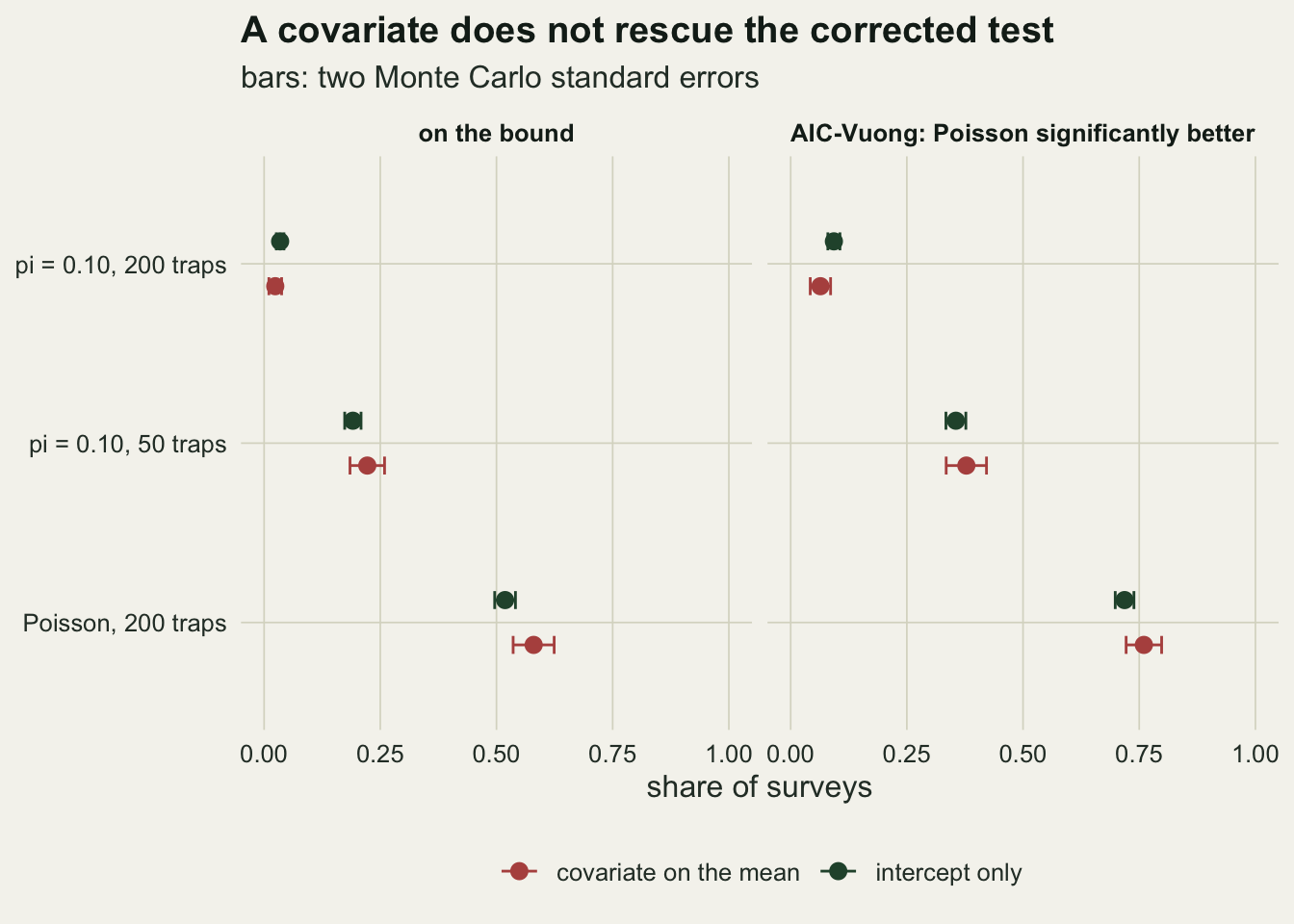
What to use instead
The first choice is the one-sided score test of van den Broek (1995). It needs no zero-inflated fit at all: from the count of zeros, the mean and, with covariates, the fitted Poisson means, it compares the observed zeros with the zeros the Poisson predicts and scales the difference by its variance. In the intercept-only case the statistic is (n0 / exp(-ybar) - n) divided by the square root of n (1 - exp(-ybar)) / exp(-ybar) - n ybar, referred to the upper 5 per cent point of a standard normal, and it rejects only when the score is positive, which is exactly when the zero-inflated fit is off the bound. In the grid above it held its size and matched the boundary likelihood ratio test in every intercept-only cell to within 9 surveys in 2000. Its two-sided version, which also rejects when there are too few zeros, held its size as well (0.050, 0.043 and 0.049 under the Poisson) but found a tenth of dead traps among 200 in 0.453 of surveys against 0.581 for the one-sided test; the direction of the question is known before the data are seen, so the one-sided test is the one to use. With the covariate the two tests had the same size under a Poisson truth with 200 traps (0.046 and 0.046), but with a tenth of traps dead the score test trailed the boundary likelihood ratio test at 200 traps (0.604 against 0.694; the likelihood ratio test alone rejected in 57 surveys and the score test alone in 12), while at 50 traps the two were level (0.244 and 0.242). So once a zero-inflated fit with covariates is at hand, the boundary likelihood ratio test is the better choice, and the score test stays the check that needs no fit. Pick one before looking at either result: with the covariate, rejecting whenever either test rejected raised the size under a Poisson truth to 0.062.
The second is the likelihood ratio test with its boundary respected: the naive chi-squared p-value halved, or equivalently the critical value taken at the 90 per cent point of a chi-squared on one degree of freedom for a 5 per cent test. The derivation and a parametric bootstrap check of it, for the negative binomial against the Poisson, are in the parametric bootstrap post; the same halving applies here because the zero-inflation probability has one boundary at zero just as the negative binomial’s inverse dispersion does. The naive test without the halving keeps its size below 5 per cent but wastes power: its size under the Poisson ran from 0.014 to 0.026, and its power at 200 traps with a tenth dead was 0.447 against 0.577 with the halving.
The third asks the same question by simulation. The check in GLM residual diagnostics simulates datasets from the fitted non-inflated model and asks whether the observed number of zeros falls outside what they produce, which is a parametric bootstrap version of the score test’s comparison and works for any family that can be simulated.
Finally, the advice in the zero-inflated models post to use information criteria survives this test. Plain AIC is a likelihood ratio test at a threshold of 2, with an asymptotic size of 0.079 rather than 0.05 (0.062 to 0.079 in the runs above), and its power at 200 traps with a tenth dead was 0.664; it can prefer the Poisson on zero-inflated data, but that preference says only that the extra parameter did not earn its penalty of 2, never that the Poisson is significantly better. The AIC-corrected Vuong test and a plain AIC comparison are different procedures with opposite behaviour here, and the names are easy to confuse.
What to report
Report which test was used for the zero-inflation question, and if it was the Vuong test from pscl, say which of the three lines was read. A significant “model2 > model1” from the AIC- or BIC-corrected line, with the Poisson as model 2, is not evidence against zero inflation.
Report the fitted zero-inflation probability and whether it sits on the boundary. For an intercept-only model that is one comparison, the observed share of zeros against exp(-ybar), and a fit on the boundary means the data carry no excess zeros relative to the Poisson with their mean, whatever any test prints.
For the test itself, report the one-sided score statistic or the boundary likelihood ratio test with its p-value computed from the 50:50 mixture, and say that the mixture was used. If the model choice was made by AIC, say so, and give the difference; a reader can then read it as a likelihood ratio test at a threshold of 2.
Honest limits
The truths here are one mean count, 1.5 beetles per working trap, two zero-inflation probabilities and three survey sizes. At higher means the Poisson predicts few zeros and a tenth of dead traps is easier to see, so all the tests should gain power and the bound should be hit less often; the forced verdict on the bound does not change, but how often it fires does. The wrong verdict inside the bound is measured, not derived, and should not be read across to other means without rerunning the code.
The covariate arm has one covariate with one slope and a zero-inflation part without covariates. The default pscl call zeroinfl(y ~ x) puts the covariate in both parts, which adds a second zero-part parameter, a penalty of two in the corrected Vuong statistics and a null hypothesis on which the zero-part slope is not identified. That case was not run, and the boundary theory used here for one parameter does not cover it directly.
The comparison is between a zero-inflated Poisson and a Poisson. With overdispersed counts the relevant pair is the zero-inflated negative binomial against the negative binomial, which has the same nesting at pi = 0 and should show the same forced verdict, but every test should have less power there, and none of those rates was measured.
The numerical fits use the optimiser, start and tolerance of pscl::zeroinfl with a finite-difference gradient, and the size of the corrected statistic on the bound depends on where BFGS stops. A fit started differently, or with the analytic gradient, would stop at a different tiny pi and print a different large negative number. The verdict would not change, because the sign and the divergence come from the algebra, not from the optimiser.
Finally, a test for zero inflation answers a narrow question: are there more zeros than this Poisson predicts. It does not say where the extra zeros come from, and a negative binomial or a missing covariate can produce the same excess, as dispersion checks for small counts notes of its own ratio.
References
Wilson P 2015 Economics Letters 127:51-53 (10.1016/j.econlet.2014.12.029)
Vuong QH 1989 Econometrica 57(2):307-333 (10.2307/1912557)
van den Broek J 1995 Biometrics 51(2):738-743 (10.2307/2532959)
Self SG, Liang KY 1987 Journal of the American Statistical Association 82(398):605-610 (10.1080/01621459.1987.10478472)