library(ggplot2)
options(scipen = 999)

te_pal <- list(forest = "#275139", green = "#2f8f63", sage = "#93a87f",
               clay = "#b5534e", gold = "#cda23f", line = "#dad9ca",
               ink = "#16241d", paper = "#f5f4ee")

theme_te <- function() {
  theme_minimal(base_size = 12) +
    theme(panel.grid.minor = element_blank(),
          panel.grid.major = element_line(colour = "#e7e6dc"),
          plot.background = element_rect(fill = "#f5f4ee", colour = NA),
          panel.background = element_rect(fill = "#f5f4ee", colour = NA),
          plot.title = element_text(face = "bold", colour = te_pal$ink),
          axis.title = element_text(colour = "#2c3a31"))
}Trophic position from stable isotopes
R
stable isotopes
trophic ecology
food webs
ecology tutorial
ggplot2
Estimate trophic position from nitrogen isotopes in R, and measure how much of a consumer’s place in the food web rests on the assumed enrichment factor.
A trophic position is a number with a decimal point in it, and that is the whole appeal. Counting links in a food web gives you integers and an argument about which links are real. Nitrogen isotopes give you a scale with decimals on it, because heavier nitrogen is retained slightly more than lighter nitrogen at every transfer, so a consumer sits a fixed distance above whatever it ate, and the distance accumulates down the chain. Divide the consumer’s excess by that fixed distance and you have a position on that scale rather than a rank.
The estimator is one line of arithmetic. What it hides is that two of the three quantities in it are not measurements of the consumer at all. The enrichment per trophic step is taken from the literature rather than from the study, and the baseline is a measurement that follows a decision about which organism represents the bottom of the chain and when to collect it. The mass spectrometer contributes a small and well characterised error to a calculation whose answer is mostly determined elsewhere. This post measures how much elsewhere, in trophic levels, with a simulation where the true trophic position is known.
If you have read Stable isotope mixing models in R the geometry here will be familiar. That post used the same isotope space to ask what proportion of a diet came from each source. This one uses it to ask how many transfers separate a consumer from the base of the web, which turns out to depend on the mixing question as well, because a consumer feeding on two food chains has two baselines and needs them weighted.
One equation, three inputs
The estimator is
\[TP = \lambda + \frac{\delta^{15}N_{c} - \delta^{15}N_{b}}{\Delta}\]
where \(\lambda\) is the trophic position of the organism chosen as the baseline, \(\delta^{15}N_{c}\) and \(\delta^{15}N_{b}\) are the consumer and baseline values, and \(\Delta\) is the trophic discrimination factor, the enrichment added at each step. The baseline is a long lived primary consumer rather than a plant or the particulate pool, because a mussel or a snail integrates several months of the plants it filters and so smooths out the week to week swings that make primary producer values almost unusable. A primary consumer sits one step above the producers, so its trophic position is fixed at two by definition rather than estimated.
Start by checking that the arithmetic does what it claims when the assumed discrimination factor is correct. The consumer is a fish with a true trophic position of 3.5. The baseline is measured as the mean of a handful of mussels, each of which varies around the true baseline value, and the consumer carries its own analytical and individual variation.
set.seed(20260718)

lambda_base <- 2
tdf_ref     <- 3.4
n15_base    <- 5.0
tp_true     <- 3.5
sd_cons     <- 0.35
sd_ind_base <- 1.00
n_base      <- 6
se_base     <- sd_ind_base / sqrt(n_base)
n15_cons_true <- n15_base + tdf_ref * (tp_true - lambda_base)

nrep <- 20000
nc <- rnorm(nrep, n15_cons_true, sd_cons)
nb <- rnorm(nrep, n15_base, se_base)
tp_hat <- lambda_base + (nc - nb) / tdf_ref

round(c(replicates = nrep, baseline_individuals = n_base, baseline_se = se_base,
        lambda = lambda_base, tdf_assumed = tdf_ref, baseline_d15N = n15_base,
        consumer_d15N = n15_cons_true, tp_true = tp_true), 4)
replicates baseline_individuals baseline_se
20000.0000 6.0000 0.4082
lambda tdf_assumed baseline_d15N
2.0000 3.4000 5.0000
consumer_d15N tp_true
10.1000 3.5000 round(c(mean_tp_hat = mean(tp_hat), bias = mean(tp_hat) - tp_true,
mc_se = sd(tp_hat) / sqrt(nrep), sd_tp_hat = sd(tp_hat)), 5)mean_tp_hat bias mc_se sd_tp_hat
3.49866 -0.00134 0.00112 0.15793 Over 20000 replicates the mean estimate is 3.49866, a bias of -0.00134 against a Monte Carlo standard error of 0.00112. The estimator is unbiased, as a linear function of two unbiased measurements has to be. The standard deviation of a single estimate is 0.15793 of a trophic level, which sounds tolerable next to the distance between one trophic level and the next.
That number is the one people quote, and it is the answer to the wrong question. It assumes the discrimination factor is exactly 3.4 and that the baseline organism is the right one, sampled at the right time. Everything below is about what happens when those two assumptions are given the uncertainty they deserve.
Here is the sampling design the rest of the post uses, drawn in the plane the measurements live in. Two primary consumers sit at the base: a pelagic filter feeder with light carbon and a benthic grazer with heavy carbon, which is the standard way of telling two food chains apart. The fish sits above and between them. The horizontal lines are the nitrogen values that integer trophic positions would occupy if the consumer’s baseline were the mixture of the two.
c_pel <- -26; c_ben <- -21
n_pel <- 5.0;  n_ben <- 9.0
alpha_true <- 0.6
n_cons <- 10
sd_cons_c <- 0.9
tp_two <- 3.5

mix_c <- alpha_true * c_pel + (1 - alpha_true) * c_ben
mix_n <- alpha_true * n_pel + (1 - alpha_true) * n_ben

set.seed(4407)
base_pts <- rbind(
  data.frame(carbon = rnorm(n_base, c_pel, sd_ind_base),
             nitrogen = rnorm(n_base, n_pel, sd_ind_base), grp = "Pelagic baseline"),
  data.frame(carbon = rnorm(n_base, c_ben, sd_ind_base),
             nitrogen = rnorm(n_base, n_ben, sd_ind_base), grp = "Benthic baseline"))
cons_pts <- data.frame(
  carbon = rnorm(n_cons, mix_c, sd_cons_c),
  nitrogen = rnorm(n_cons, mix_n + tdf_ref * (tp_two - lambda_base), sd_cons),
  grp = "Consumer")
all_pts <- rbind(base_pts, cons_pts)
all_pts$grp <- factor(all_pts$grp,
                      levels = c("Pelagic baseline", "Benthic baseline", "Consumer"))
means <- do.call(rbind, lapply(split(all_pts, all_pts$grp), function(z)
  data.frame(carbon = mean(z$carbon), nitrogen = mean(z$nitrogen),
             se_c = sd(z$carbon) / sqrt(nrow(z)), se_n = sd(z$nitrogen) / sqrt(nrow(z)),
             grp = z$grp[1])))
scale_tp <- data.frame(tp = 2:5,
                       nitrogen = mix_n + tdf_ref * ((2:5) - lambda_base))
scale_tp$lab <- paste("TP =", scale_tp$tp)

ggplot(all_pts, aes(carbon, nitrogen, colour = grp)) +
  geom_hline(data = scale_tp, aes(yintercept = nitrogen),
             colour = te_pal$line, linetype = "22", linewidth = 0.6) +
  geom_text(data = scale_tp, aes(x = -19.4, y = nitrogen + 0.35, label = lab),
            inherit.aes = FALSE, colour = "#8a8977", size = 3.1, hjust = 1) +
  geom_segment(x = c_pel, y = n_pel, xend = c_ben, yend = n_ben,
               inherit.aes = FALSE, colour = te_pal$sage, linewidth = 0.9) +
  annotate("segment", x = -25.8, y = 3.1, xend = -23.85, yend = 6.72,
           colour = "#5c6f4d", linewidth = 0.4) +
  annotate("text", x = -28.3, y = 3.0, hjust = 0, size = 3.1, colour = "#5c6f4d",
           label = "Mixture of the two baselines") +
  geom_point(size = 1.5, alpha = 0.7) +
  geom_errorbar(data = means, aes(ymin = nitrogen - se_n, ymax = nitrogen + se_n),
                width = 0, linewidth = 0.8) +
  geom_errorbar(data = means, aes(xmin = carbon - se_c, xmax = carbon + se_c),
                orientation = "y", width = 0, linewidth = 0.8) +
  geom_point(data = means, size = 4) +
  scale_colour_manual(values = c("Pelagic baseline" = te_pal$forest,
                                 "Benthic baseline" = te_pal$gold,
                                 "Consumer" = te_pal$clay), name = NULL) +
  coord_cartesian(xlim = c(-28.5, -19), ylim = c(2.5, 17.5)) +
  labs(x = "Carbon isotope ratio (per mil)", y = "Nitrogen isotope ratio (per mil)",
       title = "Two baselines and a consumer between them") +
  theme_te() +
  theme(legend.position = "top")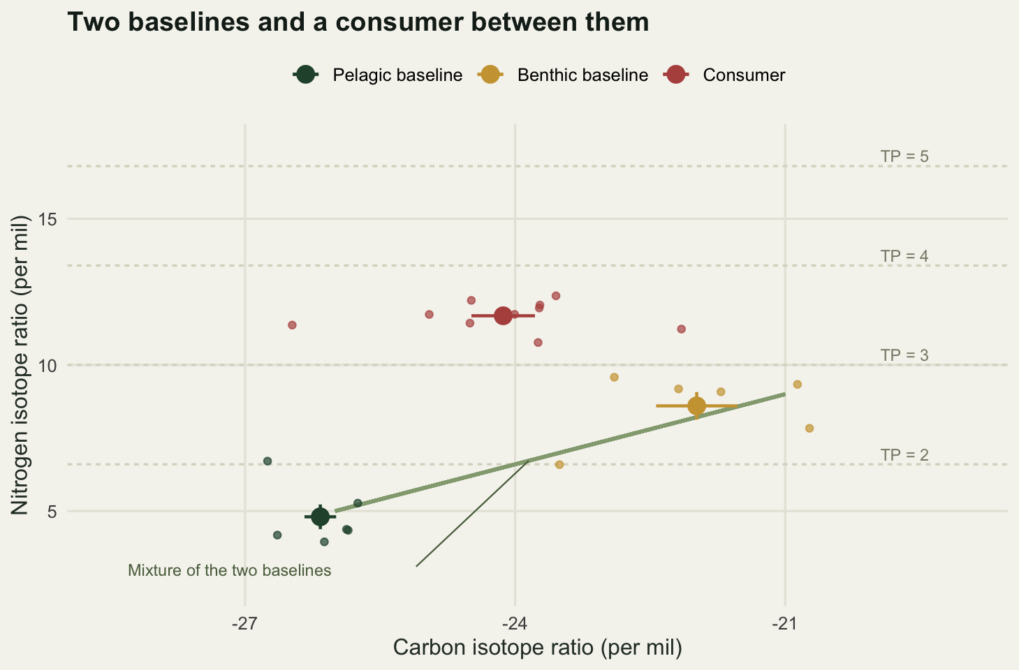
Where the uncertainty actually comes from
Write the variance of the estimate in terms of the three inputs. Because the estimator is linear in the consumer and baseline measurements, and because the excess in the numerator equals \(\Delta(TP - \lambda)\) at the truth, the first order propagation collapses to something readable:
\[\mathrm{Var}(\widehat{TP}) = \frac{\sigma_c^2 + \sigma_b^2 + (TP - \lambda)^2\,\sigma_\Delta^2}{\Delta^2}\]
The first two terms do not depend on where the consumer sits. The third does, quadratically. An error in the assumed enrichment per step is multiplied by the number of steps you are counting, so doubling a consumer’s distance above the baseline quadruples the variance that \(\Delta\) contributes and doubles the standard deviation it adds. Meta-analyses of controlled feeding studies put the standard deviation of the enrichment at roughly one per mil, which is the value used below.
We evaluate the decomposition at a low and a high trophic position, and check it against a Monte Carlo simulation in which each replicate consumer is grown with its own true enrichment drawn from that distribution while the analyst still divides by 3.4.
sd_tdf <- 1.0
var_parts <- function(tp) c(consumer = sd_cons^2, baseline = se_base^2,
                            tdf = (tp - lambda_base)^2 * sd_tdf^2) / tdf_ref^2
tp_lo <- 2.5; tp_hi <- 4.5
pa <- var_parts(tp_lo); pb <- var_parts(tp_hi)

mc_sd <- function(tp, m) {
  td  <- rnorm(m, tdf_ref, sd_tdf)
  ncc <- n15_base + td * (tp - lambda_base) + rnorm(m, 0, sd_cons)
  nbb <- rnorm(m, n15_base, se_base)
  sd(lambda_base + (ncc - nbb) / tdf_ref)
}
set.seed(11)
round(c(sd_tdf = sd_tdf, tp_low = tp_lo, tp_high = tp_hi,
        delta_sd_low = sqrt(sum(pa)), mc_sd_low = mc_sd(tp_lo, nrep),
        delta_sd_high = sqrt(sum(pb)), mc_sd_high = mc_sd(tp_hi, nrep)), 4)
sd_tdf tp_low tp_high delta_sd_low mc_sd_low
1.0000 2.5000 4.5000 0.2160 0.2167
delta_sd_high mc_sd_high
0.7521 0.7499 pct <- rbind(low = 100 * pa / sum(pa), high = 100 * pb / sum(pb))
print(round(pct, 2)) consumer baseline tdf
low 22.72 30.91 46.37
high 1.87 2.55 95.58lab_src <- c(consumer = "Consumer measurement", baseline = "Baseline measurement",
tdf = "Discrimination factor")
vd <- data.frame(
tp = rep(c(tp_lo, tp_hi), each = 3),
source = factor(rep(lab_src, 2), levels = rev(lab_src)),
pct = c(pct["low", ], pct["high", ]))
vd$panel <- factor(paste("Trophic position", vd$tp))
tops <- data.frame(panel = levels(vd$panel),
lab = paste("SD =", round(c(sqrt(sum(pa)), sqrt(sum(pb))), 3)))
ggplot(vd, aes(panel, pct, fill = source)) +
geom_col(width = 0.55) +
geom_text(data = tops, aes(panel, 104, label = lab), inherit.aes = FALSE,
colour = te_pal$ink, size = 3.6) +
scale_fill_manual(values = c("Discrimination factor" = te_pal$clay,
"Baseline measurement" = te_pal$gold,
"Consumer measurement" = te_pal$forest), name = NULL) +
coord_cartesian(ylim = c(0, 110)) +
labs(x = NULL, y = "Share of the variance (per cent)",
title = "What the error bar is made of, low and high in the web") +
theme_te() +
theme(legend.position = "top")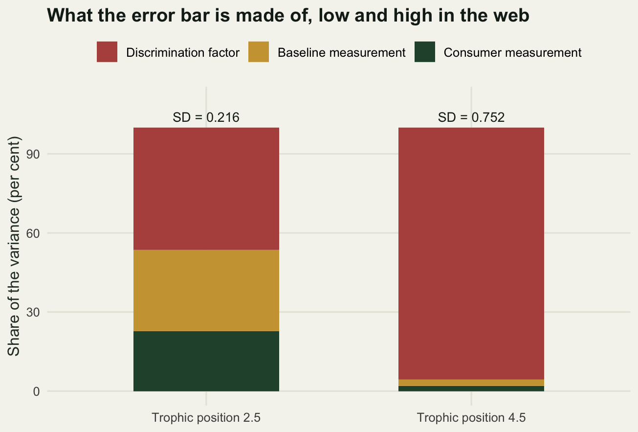
The delta method and the simulation agree: 0.216 against 0.2167 at the low trophic position, and 0.7521 against 0.7499 at the high one. The agreement is not a lucky coincidence and it is not really a check of the delta method either, because with the divisor fixed at the value the analyst chose, the estimator is exactly linear in all three inputs and the first order expansion is exact. The place where propagation stops being exact is when the divisor itself is the uncertain quantity, and no propagation formula handles that gracefully; the next section treats it as a sweep instead.
The decomposition is the result worth carrying away. At a trophic position of 2.5 the three inputs contribute 22.72, 30.91 and 46.37 per cent of the variance, so the two things you actually measured are worth more than half of it. At 4.5 the shares are 1.87, 2.55 and 95.58 per cent. For a top predator, ninety six per cent of the uncertainty in the reported trophic position comes from a number nobody in the study measured. Running more samples through the mass spectrometer, or collecting more mussels, moves the remaining four per cent.
The discrimination factor is a choice, not a measurement
Treating the enrichment as a random variable with a standard deviation is already generous, because it implies a distribution centred on the right value. In practice an analyst picks a number. The published range for nitrogen is wide, and a defensible choice can be made anywhere between about 2.5 and 4.5 per mil depending on which compilation and which taxon you lean on. Take one fixed set of measurements and sweep the assumption across that range.
tdf_grid <- seq(2.5, 4.5, by = 0.05)
cons_tp   <- c(2.5, 3.5, 4.5)
cons_n15  <- n15_base + tdf_ref * (cons_tp - lambda_base)
implied <- sapply(cons_n15, function(x) lambda_base + (x - n15_base) / tdf_grid)
colnames(implied) <- paste0("consumer_", cons_tp)

round(c(tdf_low = min(tdf_grid), tdf_high = max(tdf_grid), grid_points = length(tdf_grid)), 3)
tdf_low tdf_high grid_points
2.5 4.5 41.0 round(rbind(consumer_d15N = cons_n15,
tp_at_low_tdf = implied[1, ],
tp_at_high_tdf = implied[nrow(implied), ],
span = implied[1, ] - implied[nrow(implied), ]), 4) consumer_2.5 consumer_3.5 consumer_4.5
consumer_d15N 6.7000 10.1000 13.5000
tp_at_low_tdf 2.6800 4.0400 5.4000
tp_at_high_tdf 2.3778 3.1333 3.8889
span 0.3022 0.9067 1.5111fan <- do.call(rbind, lapply(seq_along(cons_tp), function(i)
data.frame(tdf = tdf_grid, tp = implied[, i],
consumer = sprintf("Consumer at %.1f per mil", cons_n15[i]))))
fan$consumer <- factor(fan$consumer,
levels = sprintf("Consumer at %.1f per mil", cons_n15))
ends <- fan[fan$tdf == min(tdf_grid), ]
ggplot(fan, aes(tdf, tp, colour = consumer)) +
geom_vline(xintercept = tdf_ref, colour = te_pal$line, linetype = "22",
linewidth = 0.7) +
geom_line(linewidth = 0.9) +
geom_point(data = ends, size = 2) +
scale_colour_manual(values = c(te_pal$sage, te_pal$green, te_pal$clay), name = NULL) +
labs(x = "Assumed discrimination factor (per mil)",
y = "Implied trophic position",
title = "One measurement, a whole fan of answers") +
theme_te() +
theme(legend.position = "top")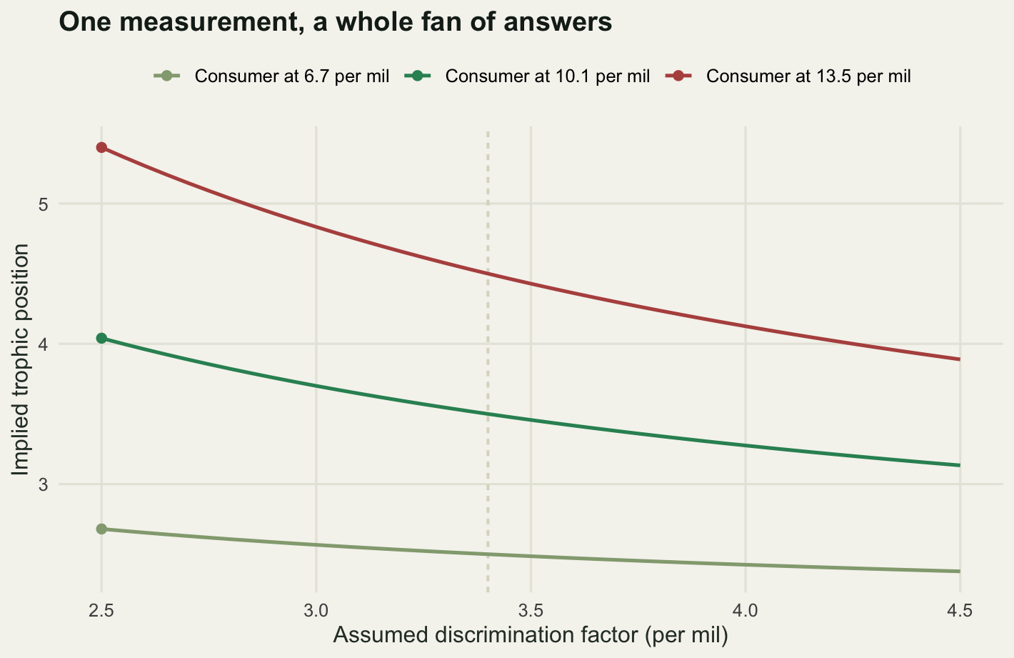
The consumer measured at 10.1 per mil is reported as a trophic position of 4.04 by an analyst who assumes 2.5, and 3.1333 by one who assumes 4.5. That is a span of 0.9067, close to a whole trophic level, from the same vial of tissue. The consumer at 13.5 per mil spans 1.5111, from 5.4 down to 3.8889, which is the difference between a top predator and a fish eating mostly invertebrates. The consumer at 6.7 per mil spans only 0.3022, because it is barely a step above its baseline and the divisor has almost nothing to divide.
The fan is the honest error bar for a trophic position, and it is far wider than the analytical one. It is also not symmetric, because the estimate is a reciprocal function of the assumption: the low end of the assumed range stretches the answer upward more than the high end compresses it.
When the enrichment depends on the diet
There is a further problem hiding inside the sweep. The enrichment is not a constant with an unknown value; it is a quantity that varies systematically with the food being eaten. Compilations of feeding experiments find that the enrichment declines as the diet itself becomes richer in heavy nitrogen, so animals eating an already enriched diet add less than animals eating a depleted one. We build a chain in which the enrichment falls by a fixed amount per unit of diet nitrogen, calibrated so that it equals 3.4 at the baseline organism’s own value, then estimate every level with the conventional constant.
tdf_slope <- 0.30
tdf_diet <- function(nd) tdf_ref - tdf_slope * (nd - n15_base)

n15_chain <- numeric(4)
n15_chain[1] <- n15_base
for (i in 1:3) n15_chain[i + 1] <- n15_chain[i] + tdf_diet(n15_chain[i])
tp_chain <- lambda_base + 0:3
tp_naive <- lambda_base + (n15_chain - n15_base) / tdf_ref

round(c(slope_per_per_mil = tdf_slope, levels = length(tp_chain)), 3)
slope_per_per_mil levels
0.3 4.0 print(round(rbind(true_tp = tp_chain, step_enrichment = tdf_diet(n15_chain),
d15N = n15_chain, estimated_tp = tp_naive,
bias = tp_naive - tp_chain), 4)) [,1] [,2] [,3] [,4]
true_tp 2.0 3.00 4.000 5.0000
step_enrichment 3.4 2.38 1.666 1.1662
d15N 5.0 8.40 10.780 12.4460
estimated_tp 2.0 3.00 3.700 4.1900
bias 0.0 0.00 -0.300 -0.8100The enrichment at the first step is 3.4 by construction, and the first estimate is therefore correct. At the next step the diet has moved up to 8.4 per mil, so the true enrichment is only 2.38, and the constant assumption reads a true trophic position of four as 3.7. At the top of the chain the step adds only 1.666, the animal sits at 12.446 per mil, and the estimate is 4.19 against a truth of five: an error of -0.81 of a trophic level.
The direction matters as much as the size. A diet dependent enrichment makes long chains look shorter than they are, because each successive step contributes less than the divisor assumes. Any comparison between systems that differ in baseline nitrogen, which includes almost every comparison between an agricultural catchment and a forested one, inherits a bias that runs the same way in both, but not by the same amount.
The slope used here, 0.3 per mil of enrichment lost per per mil of diet nitrogen, is my choice within the range these compilations report; it is not a fitted value. The point of the block is the shape of the error, not its exact size, and the shape is that it compounds upward.
Two baselines, and what mixing costs
A consumer that feeds across both food chains has no single baseline. The estimator becomes
\[TP = \lambda + \frac{\delta^{15}N_{c} - \left[\alpha\,\delta^{15}N_{b1} + (1-\alpha)\,\delta^{15}N_{b2}\right]}{\Delta}\]
with \(\alpha\) the proportion of the consumer’s nitrogen ultimately derived from the first chain. Nitrogen alone cannot supply both \(\alpha\) and \(TP\): one equation, two unknowns. Carbon does the separating, which is exactly the mixing model of the prerequisite post, and the two estimates are then joined at the hip because the carbon based \(\alpha\) feeds straight into the nitrogen baseline.
How much that coupling costs depends on how far apart the two baselines are in nitrogen. If they are identical, any error in \(\alpha\) is harmless, because both weightings give the same baseline. The further apart they are, the more a mixing error turns into a trophic position error. We measure that by replicating the whole sampling exercise for a small and a large separation.
n_ben_sep <- c(small = 5.5, large = 9.0)

two_rep <- function(nb2, m) {
  se_b <- sd_ind_base / sqrt(n_base)
  c1 <- rnorm(m, c_pel, se_b); c2 <- rnorm(m, c_ben, se_b)
  b1 <- rnorm(m, n_pel, se_b); b2 <- rnorm(m, nb2, se_b)
  mc <- alpha_true * c_pel + (1 - alpha_true) * c_ben
  mn <- alpha_true * n_pel + (1 - alpha_true) * nb2
  cc  <- rnorm(m, mc, sd_cons_c / sqrt(n_cons))
  ncn <- rnorm(m, mn + tdf_ref * (tp_two - lambda_base), sd_cons / sqrt(n_cons))
  ah <- (cc - c2) / (c1 - c2)
  th <- lambda_base + (ncn - (ah * b1 + (1 - ah) * b2)) / tdf_ref
  c(correlation = cor(ah, th), sd_alpha = sd(ah), sd_tp = sd(th),
    mean_alpha = mean(ah), mean_tp = mean(th))
}

set.seed(505)
m_two <- 6000
res_two <- rbind(small = two_rep(n_ben_sep["small"], m_two),
                 large = two_rep(n_ben_sep["large"], m_two))

round(c(replicates = m_two, consumers = n_cons, alpha_true = alpha_true,
        separation_small = as.numeric(n_ben_sep["small"] - n_pel),
        separation_large = as.numeric(n_ben_sep["large"] - n_pel)), 3)
replicates consumers alpha_true separation_small
6000.0 10.0 0.6 0.5
separation_large
4.0 print(round(res_two, 4)) correlation sd_alpha sd_tp mean_alpha mean_tp
small 0.1404 0.0842 0.0935 0.6015 3.4998
large 0.7129 0.0845 0.1353 0.6011 3.5022round(c(sd_ratio = res_two["large", "sd_tp"] / res_two["small", "sd_tp"]), 4)sd_ratio
1.4468 Both designs recover the truth: a mean \(\alpha\) of 0.6015 and 0.6011 against 0.6, and a mean trophic position of 3.4998 and 3.5022 against 3.5. The spread is what separates them. With the baselines 0.5 per mil apart the correlation between the two estimates is 0.1404 and the standard deviation of the trophic position is 0.0935. With them 4 per mil apart the correlation is 0.7129 and the spread rises to 0.1353, a factor of 1.4468.
That is the opposite of the way this is usually described, and it is worth being blunt about. The intuition says that baselines which look alike are the dangerous case, because you cannot tell which one the animal is using. The measurement says the reverse. When the baselines are close in nitrogen, \(\alpha\) is genuinely poorly determined by the nitrogen data, but it does not matter, because the trophic position barely moves as \(\alpha\) slides. When the baselines are far apart, \(\alpha\) is no better determined, and every bit of its error is amplified into the answer. The likelihood surface makes the geometry visible.
one_dataset <- function(nb2, seed) {
  set.seed(seed)
  se_b <- sd_ind_base / sqrt(n_base)
  mc <- alpha_true * c_pel + (1 - alpha_true) * c_ben
  mn <- alpha_true * n_pel + (1 - alpha_true) * nb2
  list(c1 = rnorm(1, c_pel, se_b), c2 = rnorm(1, c_ben, se_b),
       b1 = rnorm(1, n_pel, se_b), b2 = rnorm(1, nb2, se_b),
       cc = rnorm(n_cons, mc, sd_cons_c),
       nn = rnorm(n_cons, mn + tdf_ref * (tp_two - lambda_base), sd_cons))
}
a_grid <- seq(0.25, 0.95, length.out = 141)
t_grid <- seq(3.00, 4.00, length.out = 141)

surface <- function(ob) {
  gr <- expand.grid(alpha = a_grid, tp = t_grid)
  mixc <- gr$alpha * ob$c1 + (1 - gr$alpha) * ob$c2
  mixn <- gr$alpha * ob$b1 + (1 - gr$alpha) * ob$b2
  pred <- mixn + tdf_ref * (gr$tp - lambda_base)
  ssc <- (n_cons * (mixc - mean(ob$cc))^2 + sum((ob$cc - mean(ob$cc))^2)) / sd_cons_c^2
  ssn <- (n_cons * (pred - mean(ob$nn))^2 + sum((ob$nn - mean(ob$nn))^2)) / sd_cons^2
  gr$dev <- (ssc + ssn) - min(ssc + ssn)
  gr
}
ridge_line <- function(ob) data.frame(
  alpha = a_grid,
  tp = lambda_base + (mean(ob$nn) - (a_grid * ob$b1 + (1 - a_grid) * ob$b2)) / tdf_ref)

sep_levels <- c("Baselines 0.5 per mil apart", "Baselines 4 per mil apart")
ob_s <- one_dataset(n_ben_sep["small"], 24)
ob_l <- one_dataset(n_ben_sep["large"], 24)
surf <- rbind(data.frame(surface(ob_s), sep = sep_levels[1]),
              data.frame(surface(ob_l), sep = sep_levels[2]))
rl <- rbind(data.frame(ridge_line(ob_s), sep = sep_levels[1]),
            data.frame(ridge_line(ob_l), sep = sep_levels[2]))
rl <- rl[rl$tp >= min(t_grid) & rl$tp <= max(t_grid), ]
truth_pt <- data.frame(alpha = alpha_true, tp = tp_two, sep = sep_levels)
surf$sep <- factor(surf$sep, levels = sep_levels)
rl$sep <- factor(rl$sep, levels = sep_levels)
truth_pt$sep <- factor(truth_pt$sep, levels = sep_levels)

ggplot(surf, aes(alpha, tp, z = dev)) +
  geom_contour_filled(breaks = c(0, 2.3, 6.18, 11.83, Inf)) +
  geom_line(data = rl, aes(alpha, tp), inherit.aes = FALSE,
            colour = te_pal$gold, linewidth = 0.7, linetype = "22") +
  geom_point(data = truth_pt, aes(alpha, tp), inherit.aes = FALSE,
             colour = te_pal$clay, shape = 4, size = 3.4, stroke = 1.3) +
  scale_fill_manual(values = c("#275139", "#3f9970", "#93a87f", "#e6e4d6"),
                    name = "Deviance") +
  scale_x_continuous(expand = c(0, 0)) +
  scale_y_continuous(expand = c(0, 0)) +
  facet_wrap(~sep) +
  labs(x = "Mixing proportion from the pelagic chain",
       y = "Trophic position",
       title = "A ridge that only tilts when the baselines differ") +
  theme_te() +
  theme(strip.text = element_text(colour = te_pal$ink, face = "bold"),
        panel.border = element_rect(colour = "#c4c2b1", fill = NA, linewidth = 0.5),
        panel.spacing = unit(10, "pt"))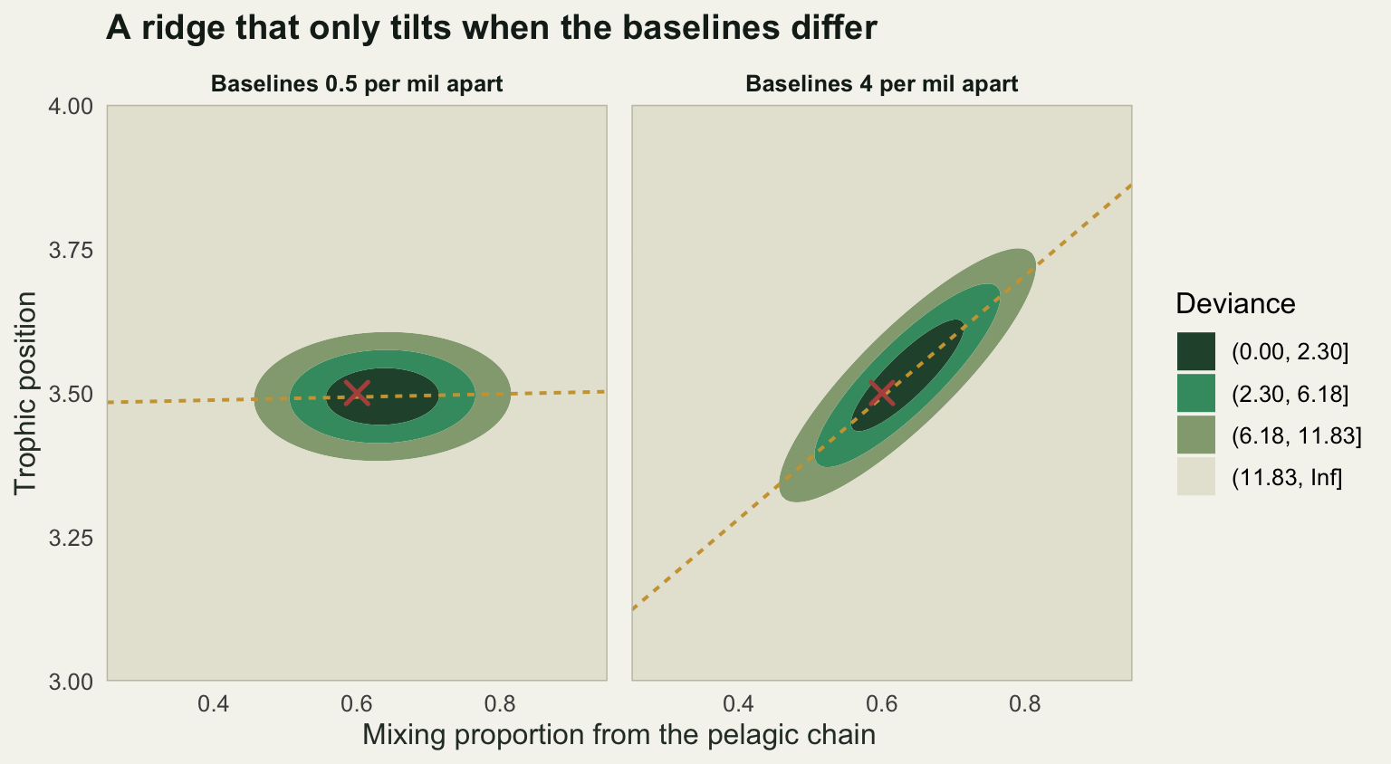
The dashed line is the whole problem in one stroke. It is the set of parameter pairs that fit the nitrogen measurements exactly, and it is what you would be left with if carbon were unavailable. In the left panel it is nearly flat, so an analyst who guessed \(\alpha\) badly would still land on close to the right trophic position. In the right panel it climbs steeply, and the shaded region tilts to follow it. Carbon cuts across that line and picks a point on it, but only as precisely as carbon itself allows, and the residual scatter travels along the tilt.
The honest limit: a baseline sampled at the wrong time
Everything above assumed the baseline number was the right number, measured with error but centred on the truth. In the field it is a bottle of mussels collected on a particular day, and baseline nitrogen moves through the year: nutrient inputs pulse, phytoplankton blooms strip the light isotope, denitrification shifts the pool. A primary consumer smooths that cycle but does not remove it, and neither does the fish, whose muscle turns over on a timescale of months and therefore records a weighted average of the past rather than the present.
Give the baseline a sinusoidal annual cycle and let the consumer’s tissue integrate it with exponential turnover. The correct baseline value to subtract is not any single day’s measurement; it is the exponentially weighted mean of the baseline over the consumer’s integration window. For a sinusoid that has a closed form: the amplitude is attenuated by a factor that depends on the ratio of the turnover rate to the annual frequency, and the phase is delayed.
amp <- 1.5
period_months <- 12
w_freq <- 2 * pi / period_months
half_life <- 2
k_turn <- log(2) / half_life
atten <- k_turn / sqrt(k_turn^2 + w_freq^2)
lag_months <- atan(w_freq / k_turn) / w_freq

phase <- 1
t_cons <- 8
base_at <- function(tt) n15_base + amp * sin(w_freq * (tt - phase))
base_eff <- n15_base + amp * atten * sin(w_freq * (t_cons - phase) - atan(w_freq / k_turn))

gaps <- seq(0, 11.99, by = 0.001)
err_gap <- (base_eff - base_at(t_cons - gaps)) / tdf_ref
best_gap <- gaps[which.min(abs(err_gap))]
off_err <- function(o) c(earlier = (base_eff - base_at(t_cons - best_gap - o)) / tdf_ref,
                         later   = (base_eff - base_at(t_cons - best_gap + o)) / tdf_ref)

round(c(amplitude = amp, period_months = period_months, half_life_months = half_life,
        turnover_rate = k_turn, attenuation = atten, phase_lag_months = lag_months), 4)
amplitude period_months half_life_months turnover_rate
1.5000 12.0000 2.0000 0.3466
attenuation phase_lag_months
0.5519 1.8833 round(c(effective_baseline = base_eff, same_day_baseline = base_at(t_cons),
same_day_tp_error = (base_eff - base_at(t_cons)) / tdf_ref,
best_gap_months = best_gap), 4)effective_baseline same_day_baseline same_day_tp_error best_gap_months
5.3694 4.2500 0.3292 1.4750 round(c(off_one_month = off_err(1), off_three_months = off_err(3),
worst_over_the_year = max(abs(err_gap)),
full_seasonal_swing = 2 * amp / tdf_ref), 4) off_one_month.earlier off_one_month.later off_three_months.earlier
-0.1992 0.2284 -0.3190
off_three_months.later worst_over_the_year full_seasonal_swing
0.5363 0.5498 0.8824 With an amplitude of 1.5 per mil and a muscle half life of two months, the consumer’s effective baseline is attenuated to 0.5519 of the seasonal amplitude and lagged by 1.8833 months. On the sampling date used here the correct baseline value is 5.3694 per mil, while a grab sample taken on the same day as the fish reads 4.25. Subtracting the wrong one inflates the trophic position by 0.3292, which is twice the analytical standard deviation measured in the first section, from a sampling decision that nobody would write down as an assumption.
Suppose instead you know about the lag and aim for the right window. Missing it by a month costs between -0.1992 and 0.2284 of a trophic level depending on which side you miss it on; missing it by three months costs between -0.319 and 0.5363. Across the whole year the worst placed baseline sample is wrong by 0.5498, and the full seasonal swing corresponds to 0.8824 of a trophic level. Those are the same magnitudes as the discrimination factor sweep, arriving from an entirely independent direction, and they add rather than cancel.
This is the limit the method cannot argue its way out of. A trophic position is a ratio of two differences, and both the numerator and the denominator are moving targets: the baseline moves through the season, and the enrichment moves with the diet. The mass spectrometer measures neither. What it does measure it measures very well, which is why the reported precision on a trophic position is almost always a statement about the instrument rather than about the food web. If a study reports a trophic position of 4.19 with a standard error in the second decimal place, the standard error is describing the tissue and the number in front of it is describing a set of assumptions.
None of this makes the method useless. It makes it a comparative method. Two consumers measured against the same baseline, in the same season, with the same assumed enrichment, differ by an amount that is very well determined, because the shared assumptions cancel in the difference. The absolute value is the fragile part, and it is the absolute value that gets quoted.
Where to go next
The sensible response to a fragile point estimate is to carry the assumptions through explicitly rather than to pick better ones. A Bayesian treatment with a prior on the enrichment and on the baseline, propagated to a posterior for the trophic position, gives an interval that reflects the fan in the third figure rather than the analytical error alone, and the same machinery handles the mixing proportion at the same time. Stable isotope mixing models in R is where that machinery is built. If your question is about niche breadth rather than chain length, the isotopic niche posts in this cluster work in the same plane with the same caveats about baselines.
References
Post DM 2002 Ecology 83(3):703-718 (10.1890/0012-9658(2002)083[0703:USITET]2.0.CO;2)
Vander Zanden MJ, Rasmussen JB 2001 Limnology and Oceanography 46(8):2061-2066 (10.4319/lo.2001.46.8.2061)
Vanderklift MA, Ponsard S 2003 Oecologia 136(2):169-182 (10.1007/s00442-003-1270-z)
Caut S, Angulo E, Courchamp F 2009 Journal of Applied Ecology 46(2):443-453 (10.1111/j.1365-2664.2009.01620.x)
Cabana G, Rasmussen JB 1996 Proceedings of the National Academy of Sciences 93(20):10844-10847 (10.1073/pnas.93.20.10844)