library(ggplot2)

te_pal <- list(forest = "#275139", green = "#2f8f63", sage = "#93a87f",
               clay = "#b5534e", gold = "#cda23f", line = "#dad9ca",
               ink = "#16241d", paper = "#f5f4ee")

theme_te <- function() {
  theme_minimal(base_size = 12) +
    theme(panel.grid.minor = element_blank(),
          panel.grid.major = element_line(colour = "#e7e6dc"),
          plot.background = element_rect(fill = "#f5f4ee", colour = NA),
          panel.background = element_rect(fill = "#f5f4ee", colour = NA),
          plot.title = element_text(face = "bold", colour = te_pal$ink),
          axis.title = element_text(colour = "#2c3a31"))
}Isotopic niche width: hulls and ellipses
R
stable isotopes
trophic ecology
ecology tutorial
ggplot2
Measure isotopic niche width in R with Layman convex hulls and standard ellipses, and see why hull area follows sample size while corrected SEAc does not.
A stable isotope biplot is one of the few pictures in trophic ecology that a whole audience reads the same way. Carbon on the horizontal axis, nitrogen on the vertical, one point per individual, and a cloud whose position says something about the diet and whose spread says something about how varied that diet is. The spread is the isotopic niche width, and the moment anyone wants to compare two groups, that spread has to become a number.
Two families of number are in general use. The first is Layman’s total area: draw the convex hull around the points and measure the polygon. The second is the bivariate standard ellipse: take the covariance matrix of the two isotope values and report the area of the ellipse it defines, with a small-sample correction applied. Both are areas in the same units, both are reported in the same sentence in hundreds of papers, and they behave completely differently when the sample size changes. That difference is the subject of this post, and it is not a detail. It decides which of two groups you conclude has the wider niche.
Everything below is simulated, so the true niche width is known in closed form and every estimate can be scored against it. If you have read home ranges in R: MCP versus kernel density the machinery will be familiar: the minimum convex polygon there is the same convex hull, and the kernel density there is the same two-dimensional density argument, moved from geographic space into isotope space. The sample-size problem is also the same problem, which is worth holding onto, because it means the answer is not a quirk of isotope work.
What the standard ellipse actually is
Take a group of consumers whose two isotope values follow a bivariate normal distribution with covariance matrix \(\Sigma\). The standard ellipse is the set of points at squared Mahalanobis distance one from the centre, which is the one-sigma contour. Its semi-axes are the square roots of the eigenvalues of \(\Sigma\), so its area is
\[\text{SEA} = \pi \sqrt{\lambda_1 \lambda_2} = \pi \sqrt{\det \Sigma}.\]
That closed form is what makes the ellipse worth simulating. There is a right answer, it can be written down, and any estimator can be held against it. The convex hull has no such thing: the convex hull of a bivariate normal population is the whole plane, so the total area has no finite population value to converge to at all. Keep that asymmetry in mind, because most of what follows falls out of it.
The simulated consumer group has a carbon standard deviation of 1.2 per mille, a nitrogen standard deviation of 0.8 per mille and a correlation of 0.15 between them, which is a modest and entirely ordinary amount of within-group variation for a fish or an invertebrate consumer sampled at one site. The estimators are three lines of base R each. The hull area is the shoelace formula applied to the vertices that chull returns; the ellipse area is the determinant of the sample covariance matrix, with cov using the usual divisor of \(n - 1\); the corrected version multiplies by \((n-1)/(n-2)\).
set.seed(20260718)

rbvn <- function(n, mu, S) {
  L <- chol(S)
  matrix(rnorm(2 * n), ncol = 2) %*% L + matrix(mu, n, 2, byrow = TRUE)
}

sea_hat  <- function(x) pi * sqrt(det(cov(x)))
seac_hat <- function(x) sea_hat(x) * (nrow(x) - 1) / (nrow(x) - 2)

hull_area <- function(x) {
  h <- chull(x)
  p <- x[h, , drop = FALSE]
  m <- nrow(p)
  k <- c(2:m, 1)
  abs(sum(p[, 1] * p[k, 2] - p[k, 1] * p[, 2])) / 2
}

sd_c <- 1.2; sd_n <- 0.8; rho <- 0.15
Sig <- matrix(c(sd_c^2, rho * sd_c * sd_n, rho * sd_c * sd_n, sd_n^2), 2)
mu_a <- c(-24.5, 9.2)
sea_true <- pi * sqrt(det(Sig))

n_huge <- 2e6
x_huge <- rbvn(n_huge, mu_a, Sig)
cen_huge <- matrix(colMeans(x_huge), n_huge, 2, byrow = TRUE)
maha <- rowSums(((x_huge - cen_huge) %*% solve(Sig)) * (x_huge - cen_huge))

round(c(sd_carbon = sd_c, sd_nitrogen = sd_n, correlation = rho,
        det_Sigma = det(Sig), SEA_true = sea_true), 5)
sd_carbon sd_nitrogen correlation det_Sigma SEA_true
1.20000 0.80000 0.15000 0.90086 2.98181 round(c(huge_sample = n_huge, SEA_huge = sea_hat(x_huge),
percent_of_truth = 100 * sea_hat(x_huge) / sea_true,
inside_ellipse_percent = 100 * mean(maha <= 1),
expected_inside_percent = 100 * (1 - exp(-0.5))), 4) huge_sample SEA_huge percent_of_truth
2000000.0000 2.9834 100.0537
inside_ellipse_percent expected_inside_percent
39.3628 39.3469 The true standard ellipse area is 2.98181 square per mille units. Estimated from a sample of two million individuals the same quantity comes back as 2.9834, which is 100.0537 per cent of the truth, so the estimator is doing what the algebra says. The ellipse also holds 39.3628 per cent of those two million individuals, against the 39.3469 per cent that \(1 - e^{-1/2}\) predicts. This is the point that gets lost in the phrase “niche width”: the standard ellipse is not a boundary of the niche. It is a contour containing about two fifths of the population, chosen because its area is a clean function of the covariance matrix.
One sample, one hull, one ellipse
Here is a single group of 40 individuals from that distribution, with both summaries drawn on it.
n_one <- 40
set.seed(707)
x_one <- rbvn(n_one, mu_a, Sig)

round(c(n = n_one, TA = hull_area(x_one), SEA = sea_hat(x_one),
        SEAc = seac_hat(x_one), SEA_true = sea_true,
        SEAc_percent_of_truth = 100 * seac_hat(x_one) / sea_true), 4)
n TA SEA
40.0000 12.1605 2.7895
SEAc SEA_true SEAc_percent_of_truth
2.8629 2.9818 96.0124 ellipse_path <- function(ce, S, npt = 200) {
th <- seq(0, 2 * pi, length.out = npt)
ee <- eigen(S)
p <- cbind(cos(th), sin(th)) %*% t(ee$vectors %*% diag(sqrt(ee$values)))
data.frame(x = p[, 1] + ce[1], y = p[, 2] + ce[2])
}
pts_one <- data.frame(carbon = x_one[, 1], nitrogen = x_one[, 2])
hull_one <- pts_one[c(chull(x_one), chull(x_one)[1]), ]
fit_one <- ellipse_path(colMeans(x_one), cov(x_one))
true_one <- ellipse_path(colMeans(x_one), Sig)
ggplot(pts_one, aes(carbon, nitrogen)) +
geom_polygon(data = hull_one, fill = te_pal$sage, alpha = 0.25,
colour = te_pal$forest, linewidth = 0.7) +
geom_path(data = true_one, aes(x, y), inherit.aes = FALSE,
colour = te_pal$ink, linetype = "22", linewidth = 0.7) +
geom_path(data = fit_one, aes(x, y), inherit.aes = FALSE,
colour = te_pal$clay, linewidth = 1) +
geom_point(colour = te_pal$forest, size = 2, alpha = 0.9) +
labs(x = "delta 13C (per mille)", y = "delta 15N (per mille)",
title = "The hull holds everything, the ellipse holds two fifths") +
theme_te()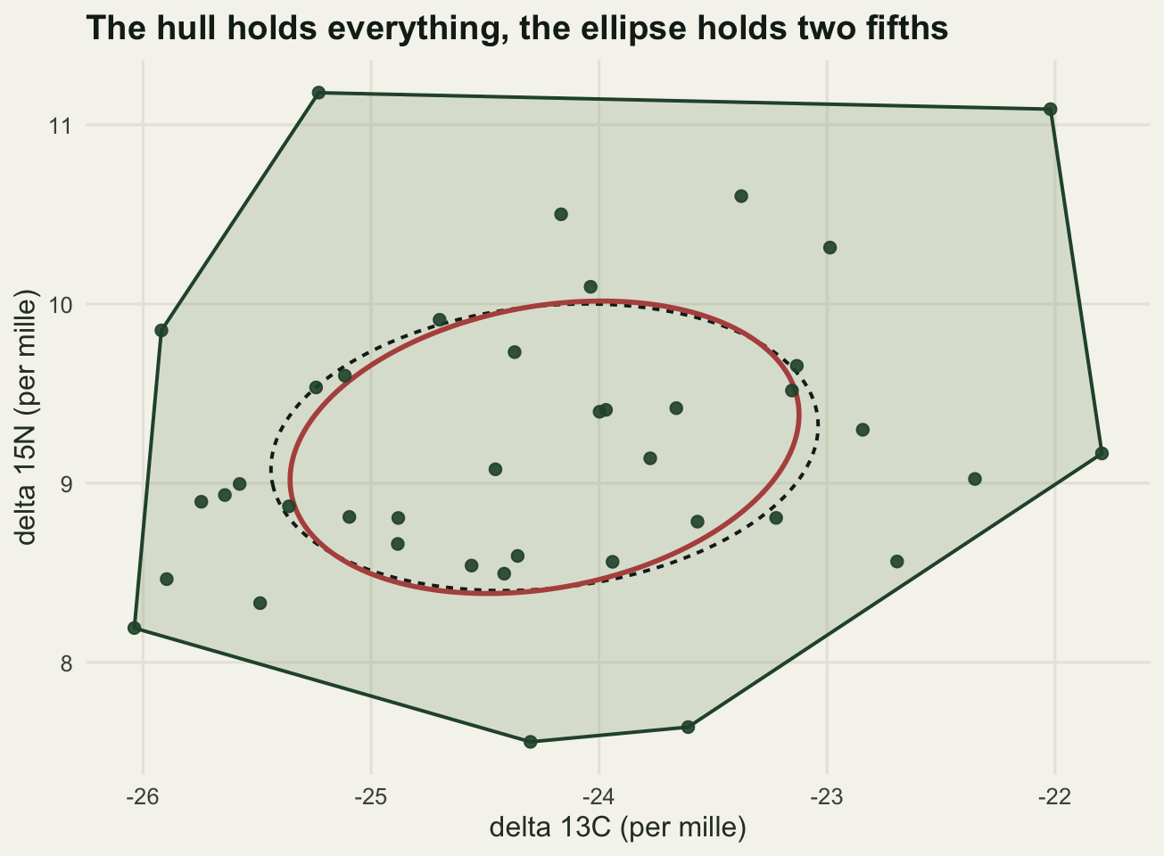
The hull area for this sample is 12.1605 and the corrected ellipse area is 2.8629, which is 96.0124 per cent of the true 2.98181. The two numbers are not comparable and were never meant to be: the hull encloses every individual including the two most extreme, while the ellipse encloses the middle of the cloud. Reporting both is fine. Comparing a hull from one paper to an ellipse from another is not, and neither is comparing two hulls without first asking how many animals went into each.
What happens as the sample grows
The sweep below draws 4000 independent groups at each of six sample sizes and averages the three metrics. Nothing about the underlying population changes across the sweep: the covariance matrix is identical at every sample size, so the true niche width is a constant, and any movement in a metric is the metric responding to the number of animals rather than to the animals.
set.seed(11)
n_seq <- c(10, 20, 40, 80, 160, 320)
n_rep <- 4000

sw <- do.call(rbind, lapply(n_seq, function(nn) {
  ta <- numeric(n_rep); se <- numeric(n_rep)
  for (i in seq_len(n_rep)) {
    x <- rbvn(nn, mu_a, Sig)
    ta[i] <- hull_area(x)
    se[i] <- sea_hat(x)
  }
  data.frame(n = nn, TA = mean(ta), SEA = mean(se),
             SEAc = mean(se) * (nn - 1) / (nn - 2))
}))
sw$TA_over_SEAtrue <- sw$TA / sea_true
sw$SEA_pct <- 100 * sw$SEA / sea_true
sw$SEAc_pct <- 100 * sw$SEAc / sea_true

print(round(sw, 4))
n TA SEA SEAc TA_over_SEAtrue SEA_pct SEAc_pct
1 10 5.1146 2.6587 2.9911 1.7153 89.1654 100.3111
2 20 8.2393 2.8195 2.9762 2.7632 94.5580 99.8112
3 40 11.5996 2.9096 2.9862 3.8901 97.5785 100.1464
4 80 15.1757 2.9490 2.9868 5.0894 98.8997 100.1677
5 160 18.8304 2.9660 2.9848 6.3151 99.4692 100.0988
6 320 22.5174 2.9714 2.9808 7.5516 99.6513 99.9646round(c(replicates = n_rep,
TA_ratio_320_over_10 = sw$TA[6] / sw$TA[1],
TA_monotone = as.numeric(all(diff(sw$TA) > 0)),
TA_last_step_percent = 100 * (sw$TA[6] / sw$TA[5] - 1),
SEA_pct_at_10 = sw$SEA_pct[1],
SEAc_pct_at_10 = sw$SEAc_pct[1],
theory_pct_at_10 = 100 * 8 / 9), 3) replicates TA_ratio_320_over_10 TA_monotone
4000.000 4.403 1.000
TA_last_step_percent SEA_pct_at_10 SEAc_pct_at_10
19.580 89.165 100.311
theory_pct_at_10
88.889 sweep_long <- rbind(
data.frame(n = sw$n, value = sw$TA / sea_true, metric = "Convex hull area (TA)"),
data.frame(n = sw$n, value = sw$SEA / sea_true, metric = "Standard ellipse area (SEA)"),
data.frame(n = sw$n, value = sw$SEAc / sea_true, metric = "Corrected ellipse area (SEAc)"))
sweep_long$metric <- factor(sweep_long$metric, levels = c(
"Convex hull area (TA)", "Standard ellipse area (SEA)",
"Corrected ellipse area (SEAc)"))
ggplot(sweep_long, aes(n, value, colour = metric)) +
geom_hline(yintercept = 1, colour = "#a9a795", linewidth = 3.4) +
geom_line(linewidth = 0.9) +
geom_point(size = 2.4) +
annotate("text", x = 10, y = 0.66, hjust = 0, size = 3.2, colour = "#5f5e4f",
label = "The thick pale band is the truth, where a metric equals the true ellipse area") +
scale_x_log10(breaks = n_seq) +
scale_y_log10(breaks = c(0.7, 0.9, 1, 2, 4, 8)) +
scale_colour_manual(values = c(te_pal$clay, te_pal$gold, te_pal$forest), name = NULL) +
labs(x = "Individuals sampled per group",
y = "Metric divided by the true ellipse area",
title = "Only one of these three measures the population") +
theme_te() +
theme(legend.position = "top")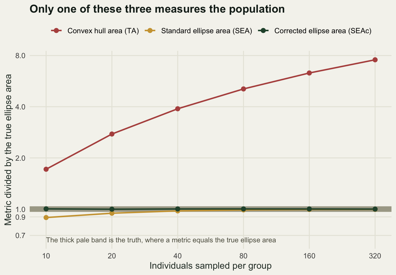
Mean hull area rises from 5.1146 at ten individuals to 22.5174 at 320, a factor of 4.403, and it rises at every step of the sweep. The last step, from 160 to 320 individuals, still adds 19.58 per cent. The percentage added by each doubling shrinks at every step, but the area added does not. There is no plateau to find because there is nothing for the hull to converge to; each new individual can only leave the polygon where it was or push it outward, so the expected area is a strictly increasing function of the sample size that grows without bound.
The ellipse behaves entirely differently, and its small-sample bias has an exact form. Writing \(S\) for the sample covariance matrix, the sampling distribution of \(\det S\) under bivariate normality factorises into two independent chi-squared variables, and taking the expectation of its square root gives
\[E[\text{SEA}] = \frac{n-2}{n-1} \, \pi \sqrt{\det \Sigma},\]
so multiplying by \((n-1)/(n-2)\) removes the bias exactly rather than approximately. At ten individuals that factor predicts a mean of 88.889 per cent of the truth. The simulation returns 89.1654 per cent, half a standard error away, and the corrected version returns 100.3111 per cent. By 320 individuals the uncorrected version has climbed to 99.6513 per cent on its own, which is why the correction is usually described as mattering only for small samples. It matters for small samples and small samples are what isotope studies have.
Two groups, two sample sizes
Now the comparison that gets made in practice. Two consumer groups are drawn from distributions with the same covariance matrix, so their true niche widths are identical to the last decimal place, and only their centres differ, as two species partitioning a food web would. One group is sampled 15 times and the other 60 times, a mismatch that is entirely normal when one species is abundant in the nets and the other is not. Over 4000 replicate pairs, how often does each metric declare the larger sample to have the wider niche?
set.seed(555)
n_small <- 15; n_big <- 60; n_pair <- 4000
mu_b <- mu_a + c(1.5, 0.6)

pair <- matrix(0, n_pair, 6)
for (i in seq_len(n_pair)) {
  a <- rbvn(n_small, mu_a, Sig)
  b <- rbvn(n_big, mu_b, Sig)
  pair[i, ] <- c(hull_area(a), hull_area(b), sea_hat(a), sea_hat(b),
                 seac_hat(a), seac_hat(b))
}
colnames(pair) <- c("TA_s", "TA_b", "SEA_s", "SEA_b", "SEAc_s", "SEAc_b")
pair <- as.data.frame(pair)

round(c(n_small = n_small, n_big = n_big, replicates = n_pair,
        TA_calls_big_wider_pct = 100 * mean(pair$TA_b > pair$TA_s),
        SEA_calls_big_wider_pct = 100 * mean(pair$SEA_b > pair$SEA_s),
        SEAc_calls_big_wider_pct = 100 * mean(pair$SEAc_b > pair$SEAc_s)), 3)
n_small n_big replicates
15.000 60.000 4000.000
TA_calls_big_wider_pct SEA_calls_big_wider_pct SEAc_calls_big_wider_pct
98.825 59.900 52.575 round(c(median_TA_ratio = median(pair$TA_b / pair$TA_s),
TA_ratio_5th_pct = as.numeric(quantile(pair$TA_b / pair$TA_s, 0.05)),
median_SEAc_ratio = median(pair$SEAc_b / pair$SEAc_s),
SEAc_ratio_5th_pct = as.numeric(quantile(pair$SEAc_b / pair$SEAc_s, 0.05)),
SEAc_ratio_95th_pct = as.numeric(quantile(pair$SEAc_b / pair$SEAc_s, 0.95))), 3) median_TA_ratio TA_ratio_5th_pct median_SEAc_ratio SEAc_ratio_5th_pct
2.036 1.192 1.021 0.639
SEAc_ratio_95th_pct
1.734 verdict <- rbind(
data.frame(ratio = pair$TA_b / pair$TA_s, metric = "Convex hull area (TA)"),
data.frame(ratio = pair$SEAc_b / pair$SEAc_s, metric = "Corrected ellipse area (SEAc)"))
verdict$metric <- factor(verdict$metric, levels = c(
"Convex hull area (TA)", "Corrected ellipse area (SEAc)"))
verdict$side <- ifelse(verdict$ratio > 1, "larger sample called wider",
"smaller sample called wider")
ggplot(verdict, aes(ratio, fill = side)) +
geom_histogram(bins = 55, colour = NA) +
geom_vline(xintercept = 1, colour = te_pal$ink, linetype = "22", linewidth = 0.7) +
facet_wrap(~metric) +
scale_x_log10(breaks = c(0.5, 1, 2, 4, 8)) +
scale_fill_manual(values = c(te_pal$clay, te_pal$green), name = NULL) +
labs(x = "Measured width of the group of 60 divided by that of the group of 15",
y = "Replicate pairs",
title = "The same niche, measured twice, judged twice") +
theme_te() +
theme(legend.position = "top",
strip.text = element_text(colour = te_pal$ink, face = "bold"))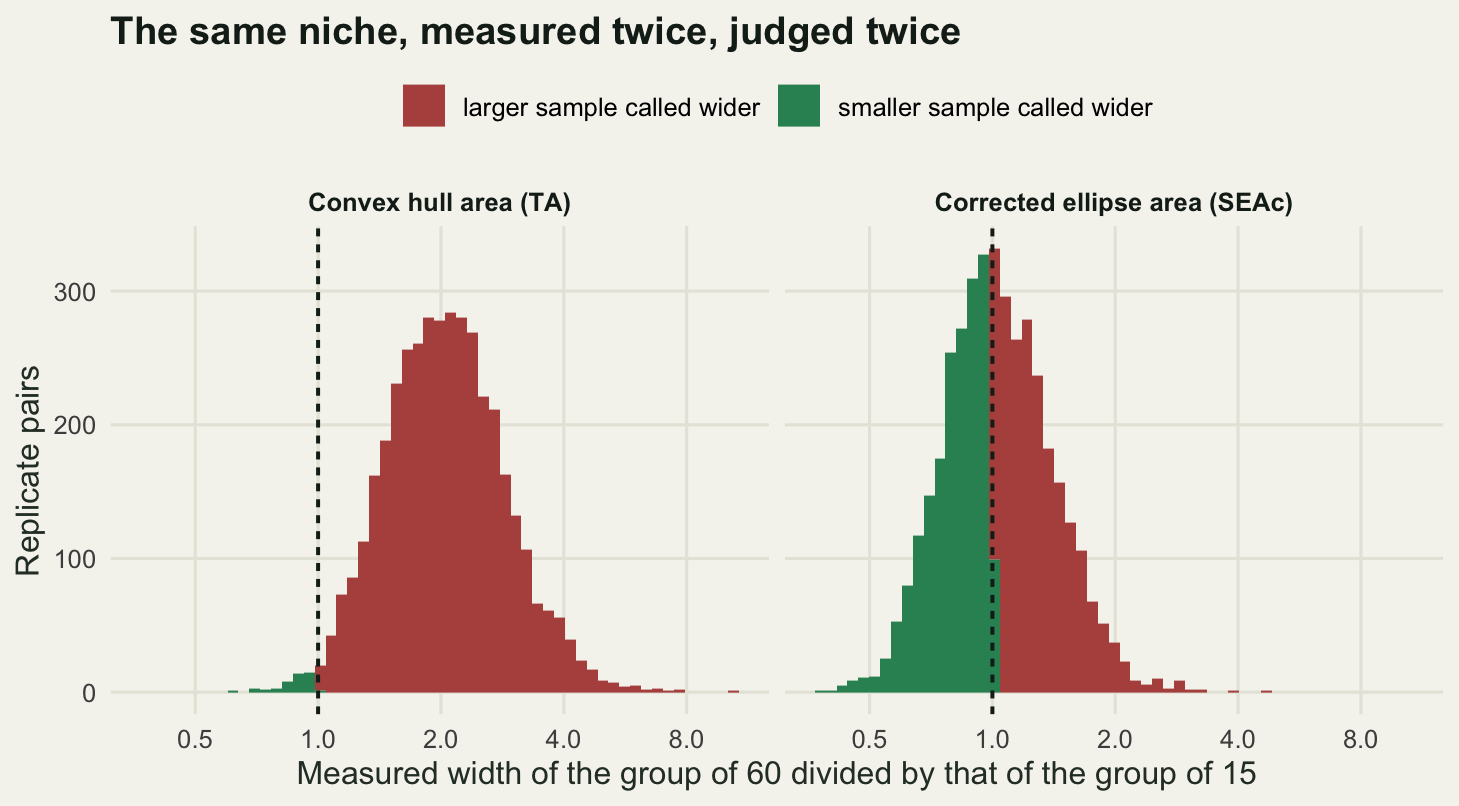
Hull area calls the larger sample wider in 98.825 per cent of the 4000 pairs. The median ratio is 2.036, and even the fifth percentile of the ratio is 1.192, so in all but the lowest twentieth of pairs the hull of the group of 60 is at least 19 per cent larger than that of the group of 15. If those were two real species you would write that the second has roughly twice the isotopic niche width of the first, and you would be reporting your sampling effort.
The corrected ellipse calls the larger sample wider in 52.575 per cent of pairs, with a median ratio of 1.021. That is the answer a metric should give when the two niches are the same. The uncorrected version sits between them at 59.9 per cent, so about a fifth of the hull’s problem survives in an uncorrected SEA and the one-line correction removes it.
Two things about the ellipse result deserve to be said rather than smoothed over. The first is that 52.575 is not fifty. The correction makes the ellipse area unbiased in its mean, which is not the same as making the comparison a coin toss: the sampling distribution of an area is skewed to the right, more so at 15 individuals than at 60, so the estimate from the smaller group falls below its own mean more often than the estimate from the larger one, which tips the count slightly. The residual tilt is a couple of percentage points, against the hull’s near certainty.
The second is the spread. The fifth to ninety-fifth percentile of the SEAc ratio runs from 0.639 to 1.734 even though the true ratio is exactly one. An unbiased metric on 15 animals is still a noisy metric on 15 animals, and a single pair of point estimates that differ by a third is weak evidence of anything. This is where the Bayesian version of the standard ellipse earns its place: fitting the covariance matrix with a posterior rather than a point estimate gives you that spread directly, per group, instead of leaving you to guess at it.
The other Layman metrics under the same sweep
Total area is one of six community-wide metrics in the original Layman set. Three others describe a single group: the mean distance of individuals to their own centroid, which is meant to capture trophic diversity; the mean nearest neighbour distance, which is meant to capture how densely packed the individuals are; and the standard deviation of those nearest neighbour distances, which is meant to capture how evenly they are packed. Each one goes through the same sweep, with 400 replicates at each sample size.
set.seed(99)
n_lay <- 400

lay <- do.call(rbind, lapply(n_seq, function(nn) {
  m <- t(replicate(n_lay, {
    x <- rbvn(nn, mu_a, Sig)
    ce <- colMeans(x)
    cd <- mean(sqrt((x[, 1] - ce[1])^2 + (x[, 2] - ce[2])^2))
    dd <- as.matrix(dist(x))
    diag(dd) <- Inf
    nnv <- apply(dd, 1, min)
    c(CD = cd, NND = mean(nnv), SDNND = sd(nnv))
  }))
  data.frame(n = nn, t(round(colMeans(m), 4)))
}))

cd_true <- mean(sqrt(rowSums((x_huge - cen_huge)^2)))
print(lay)
n CD NND SDNND
1 10 1.2002 0.6690 0.3995
2 20 1.2299 0.4796 0.3336
3 40 1.2547 0.3415 0.2555
4 80 1.2504 0.2474 0.2045
5 160 1.2626 0.1788 0.1592
6 320 1.2625 0.1283 0.1222round(c(replicates = n_lay, CD_true = cd_true,
CD_ratio_320_over_10 = lay$CD[6] / lay$CD[1],
NND_ratio_320_over_10 = lay$NND[6] / lay$NND[1],
SDNND_ratio_320_over_10 = lay$SDNND[6] / lay$SDNND[1]), 4) replicates CD_true CD_ratio_320_over_10
400.0000 1.2642 1.0519
NND_ratio_320_over_10 SDNND_ratio_320_over_10
0.1918 0.3059 Mean distance to centroid is nearly flat: 1.2002 at ten individuals and 1.2625 at 320, a ratio of 1.0519, against a population value of 1.2642 measured on the two million individual sample. It has a small downward bias at tiny samples, because the centroid is estimated from the same points it is measuring distances to, and that is the whole of the problem. Of the four metrics in this post it is the only one besides SEAc that answers a question about the population rather than about the field season.
The two nearest neighbour metrics move the other way, and they move hard. Mean nearest neighbour distance falls from 0.669 to 0.1283, which is 0.1918 of its starting value, and the standard deviation of those distances falls to 0.3059 of its starting value. This is not subtle and it is not surprising once stated: pack more points into the same region and each one finds a closer neighbour. Any comparison of nearest neighbour distances between groups of unequal size is measuring the sample sizes, in the opposite direction to the hull. A group sampled twice as hard will look as though it has a wider niche by total area and a more tightly packed one by nearest neighbour distance, from the same points.
The honest limit: one ellipse over two feeding modes
The sample-size problem has a fix. This one does not, and it is the reason to keep looking at the biplot after computing the summary.
Both metrics assume the group occupies one connected region. Suppose instead that a population feeds in two discrete ways: some individuals take a benthic diet and some a pelagic one, with almost nobody in between, which is the classic polymorphism that isotope work is used to find. The group below is built as a fifty-fifty mixture of two modes offset along the carbon axis, with the within-mode covariance chosen so that the overall covariance matrix is exactly the \(\Sigma\) used everywhere else in this post. The bimodal group therefore has the same true standard ellipse area as the unimodal one, by construction. Only the shape of the occupancy differs.
To measure what the ellipse then claims, scatter points uniformly inside the fitted standard ellipse and ask, for each, whether any actual individual lies within 0.3 per mille of it. That radius is small in isotope terms: it is a quarter of the carbon standard deviation of the group as a whole, and comparable to the analytical precision quoted for a mass spectrometer run. The proportion of the ellipse with no individual nearby is the proportion of the reported niche that nothing in the sample actually occupies.
d_sep <- 1.16
Sw <- Sig - d_sep^2 * matrix(c(1, 0, 0, 0), 2)

sim_bimodal <- function(n) {
  s <- sample(c(-1, 1), n, TRUE)
  rbvn(n, c(0, 0), Sw) + cbind(mu_a[1] + d_sep * s, mu_a[2])
}

ell_fill <- function(ce, S, m) {
  ee <- eigen(S)
  ang <- runif(m, 0, 2 * pi)
  rr <- sqrt(runif(m))
  cbind(rr * cos(ang), rr * sin(ang)) %*% t(ee$vectors %*% diag(sqrt(ee$values))) +
    matrix(ce, m, 2, byrow = TRUE)
}

uncovered <- function(x, pts, rad) {
  d2 <- outer(pts[, 1], x[, 1], "-")^2 + outer(pts[, 2], x[, 2], "-")^2
  apply(d2, 1, min) > rad^2
}

empty_share <- function(x, rad, m) {
  mean(uncovered(x, ell_fill(colMeans(x), cov(x), m), rad))
}

set.seed(4242)
n_bi <- 120; rad <- 0.3; n_bi_rep <- 120; m_grid <- 6000
emp_uni <- replicate(n_bi_rep, empty_share(rbvn(n_bi, mu_a, Sig), rad, m_grid))
emp_bi  <- replicate(n_bi_rep, empty_share(sim_bimodal(n_bi), rad, m_grid))
sea_uni <- replicate(n_bi_rep, seac_hat(rbvn(n_bi, mu_a, Sig)))
sea_bi  <- replicate(n_bi_rep, seac_hat(sim_bimodal(n_bi)))

round(c(group_n = n_bi, radius = rad, replicates = n_bi_rep, grid_points = m_grid,
        mode_offset = d_sep, modes_apart_permille = 2 * d_sep,
        within_mode_sd_carbon = sqrt(Sw[1, 1]),
        modes_apart_in_within_sd = 2 * d_sep / sqrt(Sw[1, 1])), 4)
group_n radius replicates
120.0000 0.3000 120.0000
grid_points mode_offset modes_apart_permille
6000.0000 1.1600 2.3200
within_mode_sd_carbon modes_apart_in_within_sd
0.3072 7.5510 round(c(empty_unimodal_pct = 100 * mean(emp_uni),
empty_bimodal_pct = 100 * mean(emp_bi),
ratio = mean(emp_bi) / mean(emp_uni),
SEAc_unimodal = mean(sea_uni), SEAc_bimodal = mean(sea_bi),
SEA_true = sea_true), 4)empty_unimodal_pct empty_bimodal_pct ratio SEAc_unimodal
1.3368 48.6372 36.3832 2.9785
SEAc_bimodal SEA_true
2.9553 2.9818 set.seed(88)
show_uni <- rbvn(n_bi, mu_a, Sig)
show_bi <- sim_bimodal(n_bi)
panel_lab <- c("One feeding mode", "Two feeding modes")
show_frame <- function(x, lab) {
g <- ell_fill(colMeans(x), cov(x), 4000)
gap <- uncovered(x, g, rad)
list(pts = data.frame(carbon = x[, 1], nitrogen = x[, 2], panel = lab),
hole = data.frame(carbon = g[gap, 1], nitrogen = g[gap, 2], panel = lab),
ell = data.frame(ellipse_path(colMeans(x), cov(x)), panel = lab))
}
set.seed(90)
fu <- show_frame(show_uni, panel_lab[1])
fb <- show_frame(show_bi, panel_lab[2])
bi_pts <- rbind(fu$pts, fb$pts)
bi_hole <- rbind(fu$hole, fb$hole)
bi_ell <- rbind(fu$ell, fb$ell)
for (dd in c("bi_pts", "bi_hole", "bi_ell")) {
tmp <- get(dd); tmp$panel <- factor(tmp$panel, levels = panel_lab); assign(dd, tmp)
}
bi_hole_thin <- do.call(rbind, lapply(split(bi_hole, bi_hole$panel), function(d)
d[seq(1, nrow(d), by = 2), , drop = FALSE]))
key_hole <- "Ellipse interior with no individual within 0.3 per mille"
key_ind <- "Sampled individual"
ggplot(bi_pts, aes(carbon, nitrogen)) +
geom_point(data = bi_hole_thin, aes(colour = key_hole), size = 0.55, alpha = 0.35) +
geom_path(data = bi_ell, aes(x, y), inherit.aes = FALSE,
colour = te_pal$clay, linewidth = 1) +
geom_point(aes(colour = key_ind), size = 1.6, alpha = 0.9) +
facet_wrap(~panel) +
scale_colour_manual(values = setNames(c(te_pal$gold, te_pal$forest),
c(key_hole, key_ind)),
breaks = c(key_ind, key_hole), name = NULL) +
guides(colour = guide_legend(override.aes = list(size = 2.6, alpha = 1))) +
labs(x = "delta 13C (per mille)", y = "delta 15N (per mille)",
title = "One ellipse, two very different populations",
subtitle = "The red outline is the fitted standard ellipse in both panels") +
theme_te() +
theme(legend.position = "top",
plot.subtitle = element_text(colour = "#2c3a31"),
strip.text = element_text(colour = te_pal$ink, face = "bold"))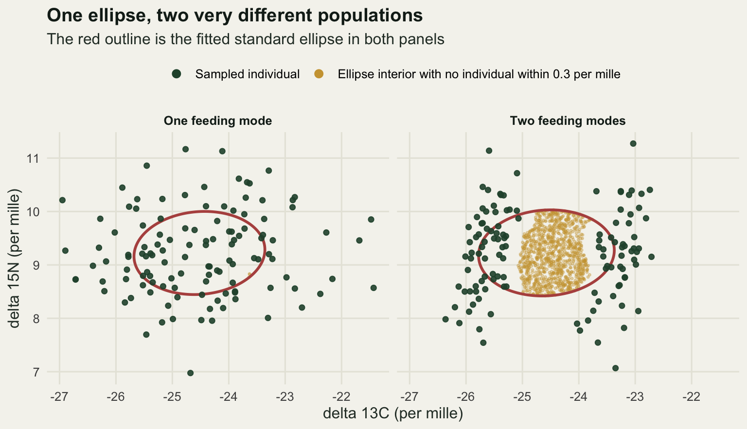
The two groups are the same size on paper. Mean corrected ellipse area is 2.9785 for the unimodal group and 2.9553 for the bimodal one, against a true 2.98181, a difference of well under a per cent and far smaller than the sampling noise measured in the previous section. Every summary statistic in this post would report them as having the same niche width, and in the sense the statistic defines, they do.
The emptiness measurement says what that costs. In the unimodal group, 1.3368 per cent of the fitted ellipse has no individual within 0.3 per mille, which is the small amount you would expect from 120 points and a finite radius. In the bimodal group it is 48.6372 per cent, a factor of 36.3832 higher. Nearly half of the reported niche is a claim about isotopic space that the sample contradicts. The two modes sit 2.3200 per mille apart along the carbon axis with a within-mode carbon standard deviation of 0.3072, which is 7.5510 within-mode standard deviations of separation, and the ellipse spans the gap as though it were occupied.
This is not a failure of the correction or of the estimator. It is what an ellipse is. A single covariance matrix has no way to express a hole, so a group that spreads out by splitting into two diets and a group that spreads out by everyone eating a bit of everything produce the same number. The consequence for interpretation is direct: a wide isotopic niche is often read as generalism at the individual level, and this construction is exactly the alternative, a population of specialists whose specialisms differ. Distinguishing them needs the biplot, or a mixture model, or repeat sampling of the same individuals through tissues with different turnover times. It does not need a better area statistic, because no area statistic can carry that information.
Where to go next
The practical rules that come out of this are short. Report the sample size beside every niche width, always. Prefer SEAc to total area for any comparison between groups, and if hull area is reported as well, say what it is doing there. Treat a difference in point estimates from small samples as weak evidence until the spread around them has been measured, which is what the Bayesian standard ellipse gives you. And look at the biplot before believing any of them.
Two groups that both have well estimated ellipses raise the next question immediately, which is how much they overlap rather than how wide each one is. That turns out to have its own sample-size trap and its own set of definitions that do not agree with each other, and it is the subject of the next post in this cluster.
References
Layman CA, Arrington DA, Montana CG, Post DM 2007 Ecology 88(1):42-48 (10.1890/0012-9658(2007)88[42:CSIRPF]2.0.CO;2)
Jackson AL, Inger R, Parnell AC, Bearhop S 2011 Journal of Animal Ecology 80(3):595-602 (10.1111/j.1365-2656.2011.01806.x)
Bearhop S, Adams CE, Waldron S, Fuller RA, Macleod H 2004 Journal of Animal Ecology 73(5):1007-1012 (10.1111/j.0021-8790.2004.00861.x)
Syvaranta J, Lensu A, Marjomaki TJ, Oksanen S, Jones RI 2013 PLoS ONE 8(2):e56094 (10.1371/journal.pone.0056094)
Swanson HK, Lysy M, Power M, Stasko AD, Johnson JD, Reist JD 2015 Ecology 96(2):318-324 (10.1890/14-0235.1)