library(ggplot2)

te_pal <- list(forest = "#275139", green = "#2f8f63", sage = "#93a87f",
               clay = "#b5534e", gold = "#cda23f", line = "#dad9ca",
               ink = "#16241d", paper = "#f5f4ee")

theme_te <- function() {
  theme_minimal(base_size = 12) +
    theme(panel.grid.minor = element_blank(),
          panel.grid.major = element_line(colour = "#e7e6dc"),
          plot.background = element_rect(fill = "#f5f4ee", colour = NA),
          panel.background = element_rect(fill = "#f5f4ee", colour = NA),
          plot.title = element_text(face = "bold", colour = te_pal$ink),
          axis.title = element_text(colour = "#2c3a31"))
}Isotopic niche overlap between groups
R
stable isotopes
trophic ecology
niche overlap
ecology tutorial
ggplot2
Code ellipse overlap for isotopic niches in R and measure how the headline percentage moves with the denominator, the containment probability and sample size.
Two groups of consumers are plotted in a carbon and nitrogen plane, and someone asks how much they overlap. The question sounds like it has one answer. It has at least three, and the difference between them is larger than the difference between most of the ecological hypotheses people use the number to separate.
The usual workflow draws a bivariate ellipse around each group and reports the shared area as a percentage. That percentage hides three decisions. The first is the denominator: overlap divided by the area of the first group is not overlap divided by the area of the second, and when one group is a generalist and the other a specialist the two answers differ by a factor of several. The second is the containment probability, which sets how much of each group’s distribution the ellipse is asked to hold. Nothing in the biology chooses it, and moving it can turn “no overlap” into “half the niche shared” for the same pair of groups. The third is what you do about sampling error, because with fifteen individuals per group the shared area is estimated so loosely that its interval covers almost the whole range it could take.
This post codes the ellipse geometry from scratch, validates the overlap calculator against two cases with known answers and a third with a closed form, and then measures all three decisions on simulated groups whose truth is known. If you have read Niche overlap: Schoener’s D and Warren’s I you have met the same question in environmental space, where the indices are built on densities over a grid rather than on a geometric shape. The isotope version differs in one way that matters: the shape is chosen by the analyst, so the analyst’s choices are inside the answer.
The ellipse, and an overlap calculator that can be checked
A group of consumers with mean \(\mu\) and covariance \(\Sigma\) in the plane of \(\delta^{13}\)C and \(\delta^{15}\)N gets a niche region defined as a level set of the squared Mahalanobis distance:
\[E(p) = \{x : (x - \mu)^{\top} \Sigma^{-1} (x - \mu) \le c_p\}, \qquad c_p = \chi^2_{2}(p)\]
Under bivariate normality that region holds a proportion \(p\) of the population, which is where the containment probability enters. Its area is \(\pi c_p \sqrt{\det \Sigma}\), so every ellipse in a study scales by the same factor \(c_p\) when \(p\) changes. That has a consequence used repeatedly below: ratios of areas do not depend on \(p\), while overlaps do.
The overlap of two ellipses has no closed form, so it has to be computed. Rather than count points on a grid, which converges slowly and leaves a ragged boundary, the calculator below slices the plane into vertical strips and solves the ellipse quadratic exactly in the second coordinate. Writing \(A = \Sigma^{-1}\) and \(u = x - \mu_1\), the boundary values of \(y\) satisfy
\[a_{22}(y - \mu_2)^2 + 2a_{12}u(y - \mu_2) + a_{11}u^2 - c_p = 0,\]
a quadratic whose two roots give the top and bottom of the ellipse at that \(x\). Two convex sets intersect in a convex set, so at each \(x\) the shared region is a single interval, and its length is the overlap of the two intervals. Integrating those lengths over \(x\) gives the area. The error is not second order in the strip width, as a midpoint rule on a smooth function would be, but of order three halves: at the two ends of the range the shared length vanishes like a square root, so its graph has a vertical tangent there, and that sets the rate rather than the curvature along the rest of the boundary.
ell_area <- function(S, p) pi * qchisq(p, 2) * sqrt(det(S))

ell_yspan <- function(x, mu, S, p) {
  cc <- qchisq(p, 2)
  A <- solve(S)
  dA <- A[1, 1] * A[2, 2] - A[1, 2]^2
  u <- x - mu[1]
  disc <- A[2, 2] * cc - dA * u^2
  half <- sqrt(pmax(disc, 0)) / A[2, 2]
  half[disc <= 0] <- NA_real_
  ctr <- mu[2] - A[1, 2] * u / A[2, 2]
  cbind(lo = ctr - half, hi = ctr + half)
}

ell_xhalf <- function(S, p) {
  cc <- qchisq(p, 2)
  A <- solve(S)
  sqrt(A[2, 2] * cc / (A[1, 1] * A[2, 2] - A[1, 2]^2))
}

ell_overlap <- function(mu1, S1, mu2, S2, p, nx = 4000) {
  h1 <- ell_xhalf(S1, p); h2 <- ell_xhalf(S2, p)
  lo <- max(mu1[1] - h1, mu2[1] - h2)
  hi <- min(mu1[1] + h1, mu2[1] + h2)
  if (hi <= lo) return(0)
  dx <- (hi - lo) / nx
  x <- lo + (seq_len(nx) - 0.5) * dx
  s1 <- ell_yspan(x, mu1, S1, p)
  s2 <- ell_yspan(x, mu2, S2, p)
  len <- pmin(s1[, "hi"], s2[, "hi"]) - pmax(s1[, "lo"], s2[, "lo"])
  len[!is.finite(len)] <- 0
  sum(pmax(len, 0)) * dx
}
A calculator nobody checks is a calculator nobody should use. Three tests, each with an answer known in advance. Two identical concentric ellipses must overlap in exactly their own area. Two ellipses pushed far apart must overlap in exactly nothing. And two circles have a classical lens formula, which tests the interesting case the first two miss: a partial overlap with a curved boundary at both ends.
n_slab <- 20000
p_ref <- 0.95
mu_g <- c(-24.0, 9.4);   S_g <- matrix(c(2.20, 0.55, 0.55, 1.35), 2)

same <- ell_overlap(mu_g, S_g, mu_g, S_g, p_ref, n_slab)
apart <- ell_overlap(mu_g, S_g, mu_g + c(50, 50), S_g, p_ref, n_slab)

lens_area <- function(r1, r2, d) {
  r1^2 * acos((d^2 + r1^2 - r2^2) / (2 * d * r1)) +
    r2^2 * acos((d^2 + r2^2 - r1^2) / (2 * d * r2)) -
    0.5 * sqrt((-d + r1 + r2) * (d + r1 - r2) * (d - r1 + r2) * (d + r1 + r2))
}
s1 <- 0.8; s2 <- 1.3; dd <- 1.9
rr <- sqrt(qchisq(p_ref, 2))
lens_true <- lens_area(s1 * rr, s2 * rr, dd)
lens_num <- ell_overlap(c(0, 0), diag(c(s1^2, s1^2)),
                        c(dd, 0), diag(c(s2^2, s2^2)), p_ref, n_slab)

c(strips = n_slab)
strips
20000 round(c(closed_form_area = ell_area(S_g, p_ref), calculator_area = same,
lens_closed_form = lens_true, lens_calculator = lens_num), 6)closed_form_area calculator_area lens_closed_form lens_calculator
30.74221 30.74221 10.15721 10.15721 signif(c(identical_relative_error = same / ell_area(S_g, p_ref) - 1,
far_apart_absolute_area = apart,
lens_relative_error = lens_num / lens_true - 1), 3)identical_relative_error far_apart_absolute_area lens_relative_error
1.10e-07 0.00e+00 1.12e-07 With 20000 strips the calculator reproduces the area of an ellipse to a relative error of 1.10e-07 and the lens area of two offset circles to 1.12e-07. Two ellipses displaced fifty units on each axis return exactly 0, because the strip range is empty and the function returns before integrating anything. That last one is worth having as a test rather than as an assumption, since a calculator that returns a small positive number for disjoint shapes will report weak overlap everywhere and nobody will notice.
Four groups, and an overlap with two answers
The rest of the post works with four consumer groups in one simulated system, specified as bivariate normals so that every “truth” below is a property of the generating distribution rather than of a sample. A generalist with a wide niche, a specialist sitting inside it, and two groups with the same niche width whose centres are separated: call them benthic and pelagic feeders, since the carbon axis is what usually separates those in a real lake.
mu_s <- c(-23.20, 9.90);  S_s <- matrix(c(0.34, 0.09, 0.09, 0.26), 2)
mu_b <- c(-25.50, 8.60);  S_b <- matrix(c(0.90, 0.25, 0.25, 0.70), 2)
mu_p <- c(-23.75, 9.95);  S_p <- S_b

p_std <- 0.40
areas <- c(generalist = ell_area(S_g, p_std), specialist = ell_area(S_s, p_std),
           benthic = ell_area(S_b, p_std), pelagic = ell_area(S_p, p_std))
round(c(containment = p_std, chisq_quantile = qchisq(p_std, 2)), 4)
containment chisq_quantile
0.4000 1.0217 round(areas, 4)generalist specialist benthic pelagic
5.2421 0.9095 2.4179 2.4179 ov_gs <- ell_overlap(mu_g, S_g, mu_s, S_s, p_std, n_slab)
round(c(shared_area = ov_gs,
divided_by_generalist = ov_gs / areas["generalist"],
divided_by_specialist = ov_gs / areas["specialist"],
ratio_of_the_two_answers = areas["generalist"] / areas["specialist"]), 4) shared_area divided_by_generalist.generalist
0.9082 0.1733
divided_by_specialist.specialist ratio_of_the_two_answers.generalist
0.9986 5.7636 At a containment probability of 0.4, which is the convention the standard ellipse in the isotope literature uses, the generalist’s ellipse covers 5.2421 units of isotope space and the specialist’s covers 0.9095. They share 0.9082 units. Divide that by the generalist and the overlap is 0.1733. Divide it by the specialist and it is 0.9986. The same pair of groups, the same shared area, and one report says the niches barely meet while the other says one group is contained in the other.
Both statements are true and they mean different things. The specialist eats a subset of what the generalist eats, so almost none of its niche is outside; the generalist eats a great deal the specialist does not, so most of its niche is unshared. The ratio between the two answers is 5.7636, and it is exactly the ratio of the two ellipse areas, because the shared area cancels. That identity is useful: if a paper reports a single overlap percentage and also reports the two ellipse areas, you can recover the number it did not give you.
ell_path <- function(mu, S, p, k = 400) {
  th <- seq(0, 2 * pi, length.out = k)
  z <- t(chol(S)) %*% rbind(cos(th), sin(th)) * sqrt(qchisq(p, 2))
  data.frame(x = mu[1] + z[1, ], y = mu[2] + z[2, ])
}

overlap_path <- function(mu1, S1, mu2, S2, p, k = 800) {
  h1 <- ell_xhalf(S1, p); h2 <- ell_xhalf(S2, p)
  lo <- max(mu1[1] - h1, mu2[1] - h2)
  hi <- min(mu1[1] + h1, mu2[1] + h2)
  if (hi <= lo) return(NULL)
  x <- seq(lo, hi, length.out = k)
  s1 <- ell_yspan(x, mu1, S1, p)
  s2 <- ell_yspan(x, mu2, S2, p)
  ylo <- pmax(s1[, "lo"], s2[, "lo"])
  yhi <- pmin(s1[, "hi"], s2[, "hi"])
  ok <- is.finite(ylo) & is.finite(yhi) & yhi > ylo
  if (!any(ok)) return(NULL)
  data.frame(x = c(x[ok], rev(x[ok])), y = c(yhi[ok], rev(ylo[ok])))
}

pan <- c("Generalist and specialist at 0.4", "Benthic and pelagic at 0.4 and 0.95")
lines_df <- rbind(
  data.frame(ell_path(mu_g, S_g, p_std), grp = "generalist", lev = "0.4", panel = pan[1]),
  data.frame(ell_path(mu_s, S_s, p_std), grp = "specialist", lev = "0.4", panel = pan[1]),
  data.frame(ell_path(mu_b, S_b, p_std), grp = "benthic", lev = "0.4", panel = pan[2]),
  data.frame(ell_path(mu_p, S_p, p_std), grp = "pelagic", lev = "0.4", panel = pan[2]),
  data.frame(ell_path(mu_b, S_b, 0.95), grp = "benthic", lev = "0.95", panel = pan[2]),
  data.frame(ell_path(mu_p, S_p, 0.95), grp = "pelagic", lev = "0.95", panel = pan[2]))
lines_df$panel <- factor(lines_df$panel, levels = pan)
lines_df$key <- paste(lines_df$grp, lines_df$lev)

fill_df <- rbind(
  data.frame(overlap_path(mu_g, S_g, mu_s, S_s, p_std), panel = pan[1]),
  data.frame(overlap_path(mu_b, S_b, mu_p, S_p, 0.95), panel = pan[2]))
fill_df$panel <- factor(fill_df$panel, levels = pan)

ggplot(lines_df, aes(x, y, group = key, colour = grp, linetype = lev)) +
  geom_polygon(data = fill_df, aes(x, y), inherit.aes = FALSE,
               fill = te_pal$gold, alpha = 0.45) +
  geom_path(linewidth = 0.8) +
  facet_wrap(~panel, scales = "free") +
  scale_colour_manual(values = c(generalist = te_pal$forest, specialist = te_pal$clay,
                                 benthic = te_pal$green, pelagic = "#c9793f"),
                      name = NULL) +
  scale_linetype_manual(values = c("0.4" = "22", "0.95" = "solid"),
                        name = "Containment") +
  labs(x = expression(delta^13 * "C (per mil)"), y = expression(delta^15 * "N (per mil)"),
       title = "Where the shared area is, and what it gets divided by") +
  theme_te() +
  theme(legend.position = "top",
        strip.text = element_text(colour = te_pal$ink, face = "bold"))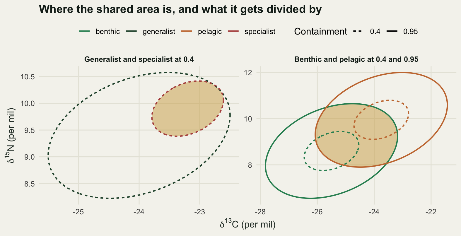
The containment probability is a free choice
Nothing about a consumer says its niche is the region holding 0.4 of its isotope distribution. That convention comes from the standard ellipse, which is the bivariate analogue of one standard deviation and is preferred because its area is less sensitive to outliers than a convex hull. Other papers set the containment to 0.95 because that is what a confidence region normally means. The choice is defensible either way and it is not a biological statement, so it should be possible to say what it costs.
Take the generalist and the benthic group, which partly overlap, and sweep the containment.
p_levels <- c(0.40, 0.60, 0.75, 0.95)
sweep_pair <- function(m1, Sa, m2, Sb, pv) {
  ov <- sapply(pv, function(p) ell_overlap(m1, Sa, m2, Sb, p, n_slab))
  data.frame(p = pv, shared = ov,
             by_first = ov / sapply(pv, function(p) ell_area(Sa, p)),
             by_second = ov / sapply(pv, function(p) ell_area(Sb, p)))
}

gb <- sweep_pair(mu_g, S_g, mu_b, S_b, p_levels)
bp <- sweep_pair(mu_b, S_b, mu_p, S_p, p_levels)
print(round(gb, 4))
p shared by_first by_second
1 0.40 0.8643 0.1649 0.3575
2 0.60 2.6354 0.2803 0.6077
3 0.75 4.9339 0.3468 0.7519
4 0.95 13.3145 0.4331 0.9390print(round(bp, 4)) p shared by_first by_second
1 0.40 0.0000 0.0000 0.0000
2 0.60 0.4816 0.1110 0.1110
3 0.75 1.5866 0.2418 0.2418
4 0.95 6.5414 0.4613 0.4613round(c(gb_extreme_ratio = max(gb$by_second) / min(gb$by_second),
bp_at_lowest_p = bp$by_second[1], bp_at_highest_p = bp$by_second[4],
bp_first_positive_p = min(bp$p[bp$shared > 0])), 4) gb_extreme_ratio bp_at_lowest_p bp_at_highest_p bp_first_positive_p
2.6267 0.0000 0.4613 0.6000 For the generalist and the benthic group the overlap as a fraction of the benthic ellipse runs 0.3575, 0.6077, 0.7519 and 0.939 across the four containment levels. The extremes differ by a factor of 2.6267. A reader handed the first number would describe two groups sharing about a third of the smaller niche; handed the last, two groups that are nearly the same. The direction is not surprising, since larger ellipses have more room to intersect, but the size of the swing is worth having in front of you: it is larger than the difference most studies are trying to detect between seasons or sexes.
Two ellipses with the same covariance touch when the Mahalanobis distance between their centres equals twice the square root of the chi-square quantile, so that threshold can be written down and compared with the separation of the benthic and pelagic groups directly.
dvec <- mu_p - mu_b
md <- sqrt(as.numeric(t(dvec) %*% solve(S_b) %*% dvec))
round(c(mahalanobis_separation = md,
        touching_separation_at_0.40 = 2 * sqrt(qchisq(0.40, 2)),
        touching_separation_at_0.95 = 2 * sqrt(qchisq(0.95, 2))), 4)
mahalanobis_separation touching_separation_at_0.40
2.1416 2.0215
touching_separation_at_0.95
4.8955 That pair is where the verdict itself flips. Their centres are 2.1416 Mahalanobis units apart. That is further apart than the 2.0215 at which two ellipses at containment 0.4 just touch, so at 0.4 they miss each other, and well inside the 4.8955 at which they would just touch at 0.95, so at 0.95 they meet. The overlap is exactly 0 at 0.4 and 0.4613 at 0.95. Nothing changed except a number in the analyst’s script.
pgrid <- seq(0.05, 0.99, by = 0.01)
curve_lab <- c("generalist and benthic, over the benthic area",
               "generalist and benthic, over the generalist area",
               "benthic and pelagic, either area")
ov_gb <- sapply(pgrid, function(p) ell_overlap(mu_g, S_g, mu_b, S_b, p, 3000))
ov_bp <- sapply(pgrid, function(p) ell_overlap(mu_b, S_b, mu_p, S_p, p, 3000))
a_g <- sapply(pgrid, function(p) ell_area(S_g, p))
a_b <- sapply(pgrid, function(p) ell_area(S_b, p))
curves <- rbind(
  data.frame(p = pgrid, value = ov_gb / a_b, series = curve_lab[1]),
  data.frame(p = pgrid, value = ov_gb / a_g, series = curve_lab[2]),
  data.frame(p = pgrid, value = ov_bp / a_b, series = curve_lab[3]))
curves$series <- factor(curves$series, levels = curve_lab)

ggplot(curves, aes(p, value, colour = series)) +
  geom_vline(xintercept = p_levels, colour = te_pal$line, linewidth = 0.7) +
  geom_line(linewidth = 0.9) +
  scale_colour_manual(values = c(te_pal$forest, te_pal$sage, te_pal$clay), name = NULL) +
  guides(colour = guide_legend(ncol = 1)) +
  labs(x = "Containment probability of the ellipse", y = "Overlap as a proportion of one area",
       title = "What the containment probability alone does to an overlap") +
  theme_te() +
  theme(legend.position = "top")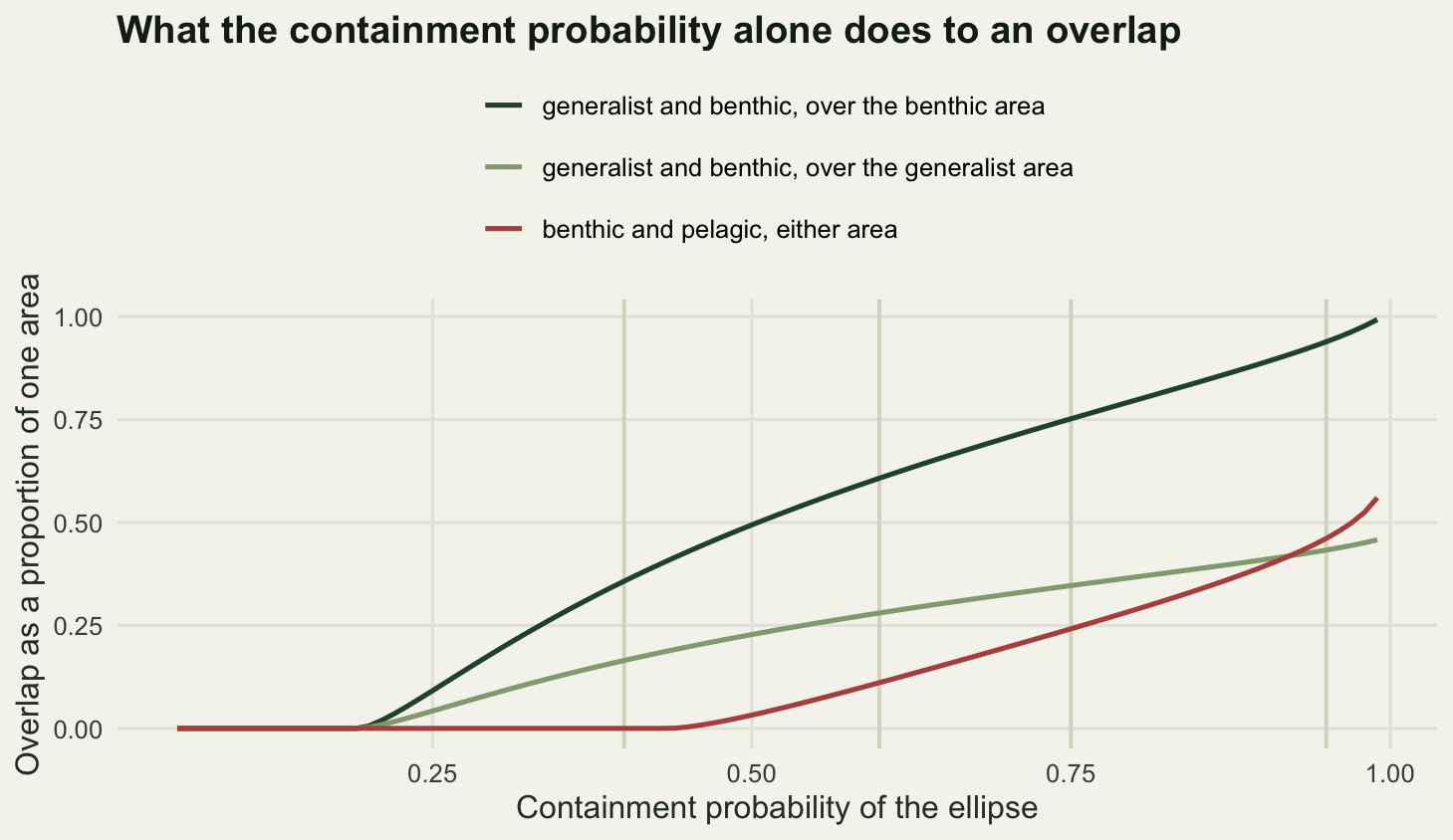
What fifteen individuals are worth
Everything so far treated the ellipses as known. In a real study each group is a sample, the mean and covariance are estimates, and the overlap is a nonlinear function of ten estimated quantities. Fifteen individuals per group is a normal isotope sample size, often a generous one. Simulate that situation many times, compute the plug-in overlap each time, and compare against the truth the data were generated from.
set.seed(20260718)
rmvn <- function(n, mu, S) t(mu + t(chol(S)) %*% matrix(rnorm(2 * n), nrow = 2))

n_ind <- 15
n_rep <- 3000
truth_prop <- ell_overlap(mu_g, S_g, mu_b, S_b, p_std, n_slab) / ell_area(S_b, p_std)
kc <- (n_ind - 1) / (n_ind - 2)

est <- numeric(n_rep); est_c <- numeric(n_rep)
for (i in seq_len(n_rep)) {
  xg <- rmvn(n_ind, mu_g, S_g); xb <- rmvn(n_ind, mu_b, S_b)
  mg <- colMeans(xg); mb <- colMeans(xb)
  Sg <- cov(xg); Sb_hat <- cov(xb)
  est[i] <- ell_overlap(mg, Sg, mb, Sb_hat, p_std, 1500) / ell_area(Sb_hat, p_std)
  est_c[i] <- ell_overlap(mg, kc * Sg, mb, kc * Sb_hat, p_std, 1500) /
    ell_area(kc * Sb_hat, p_std)
}

round(c(individuals_per_group = n_ind, replicates = n_rep,
        small_sample_factor = kc), 4)
individuals_per_group replicates small_sample_factor
15.0000 3000.0000 1.0769 round(c(truth = truth_prop, mean_estimate = mean(est), bias = mean(est) - truth_prop,
median_estimate = median(est)), 4) truth mean_estimate bias median_estimate
0.3575 0.3112 -0.0463 0.2712 round(c(interval_coverage_percent = 95,
lower_2.5 = as.numeric(quantile(est, 0.025)),
upper_97.5 = as.numeric(quantile(est, 0.975)),
interval_width = as.numeric(diff(quantile(est, c(0.025, 0.975)))),
proportion_exactly_zero = mean(est == 0),
proportion_above_0.9 = mean(est > 0.9)), 4)interval_coverage_percent lower_2.5 upper_97.5
95.0000 0.0000 0.8822
interval_width proportion_exactly_zero proportion_above_0.9
0.8822 0.1010 0.0213 round(c(corrected_mean = mean(est_c), corrected_bias = mean(est_c) - truth_prop), 4)corrected_mean corrected_bias
0.3379 -0.0196 The truth is an overlap of 0.3575 of the benthic ellipse. Across 3000 replicates of 15 individuals per group the mean estimate is 0.3112, so the plug-in estimator runs 0.0463 low, and the median is lower still at 0.2712. The central 95 per cent of the estimates runs from 0 to 0.8822, a width of 0.8822 on a quantity bounded between zero and one. In 0.101 of replicates the two sample ellipses do not touch at all and the study reports no overlap; in 0.0213 of them the overlap comes back above 0.9 and the study reports two groups eating the same thing.
That is the third decision, and it is not a decision anyone makes consciously. A point estimate of overlap from fifteen individuals per group carries essentially no information about where in the unit interval the truth sits. Two studies of the same two populations, both done properly, can report 0 and 0.8822 and neither of them has made a mistake.
The downward bias has a known partial fix. The sample covariance underestimates the population ellipse area in small samples, and the standard correction multiplies it by \((n-1)/(n-2)\), which here is 1.0769. Applying it moves the mean estimate to 0.3379 and cuts the bias from 0.0463 to 0.0196. It removes more than half of the bias and does nothing at all for the spread, which was the larger problem.
qs <- as.numeric(quantile(est, c(0.025, 0.975)))
ggplot(data.frame(est = est), aes(est)) +
  geom_histogram(binwidth = 0.025, boundary = 0, fill = te_pal$sage,
                 colour = te_pal$forest, linewidth = 0.25) +
  geom_vline(xintercept = truth_prop, colour = te_pal$ink, linewidth = 0.9) +
  geom_vline(xintercept = qs, colour = te_pal$clay, linewidth = 0.7, linetype = "22") +
  annotate("text", x = qs[2] - 0.012, y = 432, hjust = 1, size = 3.1,
           colour = te_pal$clay,
           label = "Upper bound of the central 95 per cent of estimates") +
  annotate("text", x = qs[1] + 0.03, y = 250, hjust = 0, size = 3.1,
           colour = te_pal$clay,
           label = "Lower bound, sitting at zero") +
  annotate("text", x = truth_prop + 0.018, y = 348, hjust = 0, size = 3.1,
           colour = te_pal$ink, fontface = "bold",
           label = "The truth") +
  labs(x = "Estimated overlap, proportion of the benthic ellipse", y = "Replicates",
       title = "One truth, and the answers fifteen individuals give") +
  theme_te()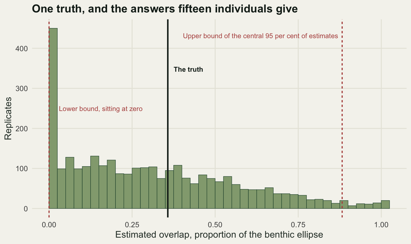
A posterior for the ordering, and what it costs
The honest response to that spread is to stop reporting a point estimate and report a distribution. The usual route puts an inverse-Wishart posterior on each group’s covariance, which with a flat reference prior is \(\Sigma \mid X \sim \text{IW}(S, n-1)\) where \(S\) is the matrix of sums of squares about the sample mean. Drawing from it needs a Wishart draw and an inverse, and for two dimensions the Bartlett decomposition writes that in four lines.
For \(W \sim \text{Wishart}(\nu, V)\) with \(V = LL^{\top}\), build a lower triangular \(A\) whose diagonal entries are square roots of chi-square draws on \(\nu\) and \(\nu - 1\) degrees of freedom and whose one off-diagonal entry is standard normal. Then \(W = LAA^{\top}L^{\top}\), and \(\Sigma = W^{-1}\) is an inverse-Wishart draw with scale \(V^{-1}\). Everything below is coded directly on the four entries of a two by two matrix so that thousands of draws cost one vectorised pass.
rinvwish2 <- function(m, S, df) {
  L <- t(chol(solve(S)))
  a11 <- sqrt(rchisq(m, df))
  a22 <- sqrt(rchisq(m, df - 1))
  a21 <- rnorm(m)
  m11 <- L[1, 1] * a11
  m21 <- L[2, 1] * a11 + L[2, 2] * a21
  m22 <- L[2, 2] * a22
  w11 <- m11^2; w12 <- m11 * m21; w22 <- m21^2 + m22^2
  dw <- w11 * w22 - w12^2
  cbind(s11 = w22 / dw, s12 = -w12 / dw, s22 = w11 / dw, det = 1 / dw)
}

set.seed(4407)
S_check <- matrix(c(9.0, 2.5, 2.5, 6.0), 2)
df_check <- 14L
n_check <- 200000L
chk <- rinvwish2(n_check, S_check, df_check)
target <- c(S_check[1, 1], S_check[1, 2], S_check[2, 2]) / (df_check - 3)
print(round(rbind(sampler = colMeans(chk[, 1:3]), analytic = target), 4))
s11 s12 s22
sampler 0.8189 0.2271 0.5448
analytic 0.8182 0.2273 0.5455c(check_df = df_check, check_draws = n_check) check_df check_draws
14 200000 signif(c(max_relative_error = max(abs(colMeans(chk[, 1:3]) / target - 1))), 2)max_relative_error
0.0012 The mean of an inverse-Wishart with scale \(S\) and \(\nu\) degrees of freedom in two dimensions is \(S/(\nu - 3)\). Over 200000 draws the sampler matches that to a maximum relative error of 0.0012 across the three distinct entries, which is the right size for the Monte Carlo error of that many draws. The sampler is correct.
Now ask the question ecologists actually ask of two niche widths: is group A narrower than group B? Ellipse area is \(\pi c_p \sqrt{\det \Sigma}\), so the comparison reduces to \(\det \Sigma_A < \det \Sigma_B\) and the containment probability drops out entirely. Unlike the overlaps above, this ordering does not move with the analyst’s choice of \(p\): comparing the determinants and comparing the two ellipse areas at any chosen level are the same question, for the same reason the ratio of two areas was free of \(p\) in the first section.
set.seed(881)
S_narrow <- 0.6 * S_b
n_draw <- 4000

post_narrower <- function(xa, xb, m) {
  da <- rinvwish2(m, (nrow(xa) - 1) * cov(xa), nrow(xa) - 1)[, "det"]
  db <- rinvwish2(m, (nrow(xb) - 1) * cov(xb), nrow(xb) - 1)[, "det"]
  mean(da < db)
}

x_narrow <- rmvn(n_ind, mu_b, S_narrow); x_wide <- rmvn(n_ind, mu_p, S_b)
y_one <- rmvn(n_ind, mu_b, S_b); y_two <- rmvn(n_ind, mu_p, S_b)

round(c(true_area_ratio = sqrt(det(S_narrow) / det(S_b)),
        posterior_draws = n_draw,
        P_narrower_when_true = post_narrower(x_narrow, x_wide, n_draw),
        P_narrower_when_equal = post_narrower(y_one, y_two, n_draw)), 4)
true_area_ratio posterior_draws P_narrower_when_true
0.6000 4000.0000 0.8118
P_narrower_when_equal
0.4542 set.seed(5150)
n_study <- 1200
pr_eq <- numeric(n_study); pr_tr <- numeric(n_study)
for (i in seq_len(n_study)) {
pr_eq[i] <- post_narrower(rmvn(n_ind, mu_b, S_b), rmvn(n_ind, mu_p, S_b), n_draw)
pr_tr[i] <- post_narrower(rmvn(n_ind, mu_b, S_narrow), rmvn(n_ind, mu_p, S_b), n_draw)
}
round(c(studies = n_study,
equal_median_P = median(pr_eq),
equal_P_above_0.95 = mean(pr_eq > 0.95),
equal_P_below_0.05 = mean(pr_eq < 0.05),
false_confidence_rate = mean(pr_eq > 0.95 | pr_eq < 0.05)), 4) studies equal_median_P equal_P_above_0.95
1200.0000 0.5145 0.0550
equal_P_below_0.05 false_confidence_rate
0.0433 0.0983 round(c(true_median_P = median(pr_tr),
true_P_above_0.95 = mean(pr_tr > 0.95),
true_wrong_side_of_half = mean(pr_tr < 0.5)), 4) true_median_P true_P_above_0.95 true_wrong_side_of_half
0.8958 0.3567 0.1025 Where group A really is narrower, by a true area ratio of 0.6, one simulated study of 15 individuals per group returns a posterior probability of 0.8118 that it is narrower. Most readers would call that suggestive and stop short of a claim, but that reading is an accident of the particular sample: repeat the sampling and the probability can come back on the wrong side of a half, or high enough to look decisive. Across 1200 such studies the median posterior probability is 0.8958, only 0.3567 of them reach 0.95, and 0.1025 of them land on the wrong side of a half, meaning they favour the ordering that is false. An area ratio of 0.6 is a large biological difference, and at this sample size roughly a third of properly conducted studies detect it with confidence.
Where the two groups are genuinely equal, the single simulated study returns 0.4542. That one number carries no information about the tie: draw a fresh sample from the same design and it can land anywhere from near zero to near one, so a value close to a half is a coincidence rather than a reassurance. Across 1200 studies, 0.055 put the probability above 0.95 and 0.0433 put it below 0.05, so 0.0983 of them make a confident directional claim about an ordering that does not exist.
That rate is almost exactly what it should be, and that is the uncomfortable part. Under an exact tie a calibrated posterior probability is close to uniform, so about a tenth of studies must land in the two five per cent tails, and the measurement sits on that value. The inverse-Wishart is not misbehaving, and no amount of care with the statistics will lower the number. Asking a directional question of a tie produces a confident wrong direction at a rate fixed by the arithmetic, and the only thing that helps is reporting the probability instead of the direction. A literature that reports “group A had the narrower isotopic niche” without the probability attached is publishing the tail of that distribution and calling it a result.
Isotope space is not niche space
The four groups above were bivariate normals with no diet behind them, which was convenient for knowing the truth and dishonest about where isotope values come from. A consumer’s signature is a mixture of what it ate, shifted by trophic discrimination. Two consumers land in the same place when their diets have the same mixture of signatures, and prey species with the same signature are common: congeners at the same trophic level, filter feeders in the same water column, grazers on the same algal mat.
So construct the extreme case. Four prey species, in two pairs with identical isotopic signatures. One consumer eats only the first member of each pair, the other only the second. Their diets share no species at all. Every individual mixes its two prey in a proportion drawn from a beta distribution, adds a trophic discrimination factor, and picks up assimilation and analytical noise.
set.seed(303)
prey_low <- c(-27.0, 6.0)
prey_high <- c(-21.5, 8.5)
tdf <- c(0.4, 3.4)
sig_ind <- matrix(c(0.16, 0.02, 0.02, 0.13), 2)
n_cons <- 60

draw_consumer <- function(n) {
  w <- rbeta(n, 2.5, 2.5)
  base <- cbind(w * prey_low[1] + (1 - w) * prey_high[1],
                w * prey_low[2] + (1 - w) * prey_high[2])
  base + t(t(chol(sig_ind)) %*% matrix(rnorm(2 * n), nrow = 2)) +
    matrix(tdf, nrow = n, ncol = 2, byrow = TRUE)
}

diet_a <- c(0.5, 0.0, 0.5, 0.0)
diet_b <- c(0.0, 0.5, 0.0, 0.5)

xa <- draw_consumer(n_cons); xb <- draw_consumer(n_cons)
Sa <- cov(xa); Sb2 <- cov(xb)
ov_ab <- ell_overlap(colMeans(xa), Sa, colMeans(xb), Sb2, p_std, n_slab)

round(c(consumers_per_group = n_cons, prey_species = length(diet_a),
        shared_prey_species = sum(diet_a > 0 & diet_b > 0),
        true_dietary_overlap = sum(pmin(diet_a, diet_b)),
        true_isotopic_overlap = 1), 4)
consumers_per_group prey_species shared_prey_species
60 4 0
true_dietary_overlap true_isotopic_overlap
0 1 round(c(measured_over_a = ov_ab / ell_area(Sa, p_std),
measured_over_b = ov_ab / ell_area(Sb2, p_std),
centroid_distance = sqrt(sum((colMeans(xa) - colMeans(xb))^2))), 4) measured_over_a measured_over_b centroid_distance
0.8606 0.8659 0.0679 set.seed(717)
n_rep2 <- 300
rep_ov <- sapply(seq_len(n_rep2), function(i) {
a <- draw_consumer(n_cons); b <- draw_consumer(n_cons)
Aa <- cov(a); Bb <- cov(b)
ell_overlap(colMeans(a), Aa, colMeans(b), Bb, p_std, 1500) / ell_area(Aa, p_std)
})
round(c(replicates = n_rep2, percentile_low = 5, percentile_high = 95,
median_measured_overlap = median(rep_ov),
lower_5 = as.numeric(quantile(rep_ov, 0.05)),
upper_95 = as.numeric(quantile(rep_ov, 0.95))), 4) replicates percentile_low percentile_high
300.0000 5.0000 95.0000
median_measured_overlap lower_5 upper_95
0.8570 0.6781 0.9859 The true dietary overlap is 0: the proportions share no prey species, so the sum of their minima is zero on all four. The true isotopic overlap is 1, because the two consumers are draws from the same generating distribution. In the simulated dataset the measured overlap is 0.8606 of the first ellipse and 0.8659 of the second, with the two centroids 0.0679 apart. Across 300 replicate studies the median measured overlap is 0.857, with a 5th to 95th percentile range of 0.6781 to 0.9859.
The measurement is not wrong. Those consumers really do occupy the same region of isotope space, and if the question were “do these two groups draw on the same energy pathways in the same proportions” the answer would be yes. The trouble is that the question people ask is about competition and resource partitioning, and on that question the measurement is maximally misleading: two consumers with no prey species in common score an overlap of 0.857. Isotope space is a two dimensional projection of a diet space with as many dimensions as there are prey types, and any projection collapses distinctions.
The corollary runs the other way too, and it is the one worth remembering when a study reports low overlap. Two consumers eating exactly the same prey species can be separated in isotope space if their prey are drawn from different places, since baseline carbon shifts along a shoreline or between a stream and its lake. Low isotopic overlap is then a statement about where the animals fed, not about what they ate. Neither direction of error is detectable from the isotope data alone. Gut contents, faecal metabarcoding or direct observation are the only things that fix it, and they are what the isotope study was usually meant to replace.
pts <- rbind(data.frame(x = xa[, 1], y = xa[, 2], grp = "consumer A: prey 1 and 3"),
             data.frame(x = xb[, 1], y = xb[, 2], grp = "consumer B: prey 2 and 4"))
ells <- rbind(
  data.frame(ell_path(colMeans(xa), Sa, p_std), grp = "consumer A: prey 1 and 3"),
  data.frame(ell_path(colMeans(xb), Sb2, p_std), grp = "consumer B: prey 2 and 4"))
shade <- overlap_path(colMeans(xa), Sa, colMeans(xb), Sb2, p_std)
mixline <- data.frame(x = c(prey_low[1], prey_high[1]) + tdf[1],
                      y = c(prey_low[2], prey_high[2]) + tdf[2])
preys <- mixline

ggplot(pts, aes(x, y, colour = grp)) +
  geom_polygon(data = shade, aes(x, y), inherit.aes = FALSE,
               fill = te_pal$gold, alpha = 0.4) +
  geom_line(data = mixline, aes(x, y), inherit.aes = FALSE,
            colour = te_pal$ink, linetype = "22", linewidth = 0.5) +
  geom_point(size = 1.6, alpha = 0.85) +
  geom_path(data = ells, aes(x, y, colour = grp), linewidth = 0.9) +
  geom_point(data = preys, aes(x, y), inherit.aes = FALSE, shape = 22,
             size = 3.4, stroke = 1.1, colour = te_pal$ink, fill = te_pal$paper) +
  annotate("text", x = min(mixline$x) - 0.15, y = max(mixline$y) + 0.34, hjust = 0,
           size = 3.0, colour = "#3d4a41",
           label = "Open squares: the two prey signatures after discrimination") +
  annotate("text", x = max(mixline$x) + 0.15, y = min(mixline$y) - 0.16, hjust = 1,
           size = 3.0, colour = "#3d4a41",
           label = "Dotted line: mixtures of those two") +
  scale_colour_manual(values = c(te_pal$forest, te_pal$clay), name = NULL) +
  labs(x = expression(delta^13 * "C (per mil)"), y = expression(delta^15 * "N (per mil)"),
       title = "Disjoint diets, one isotopic niche") +
  theme_te() +
  theme(legend.position = "top")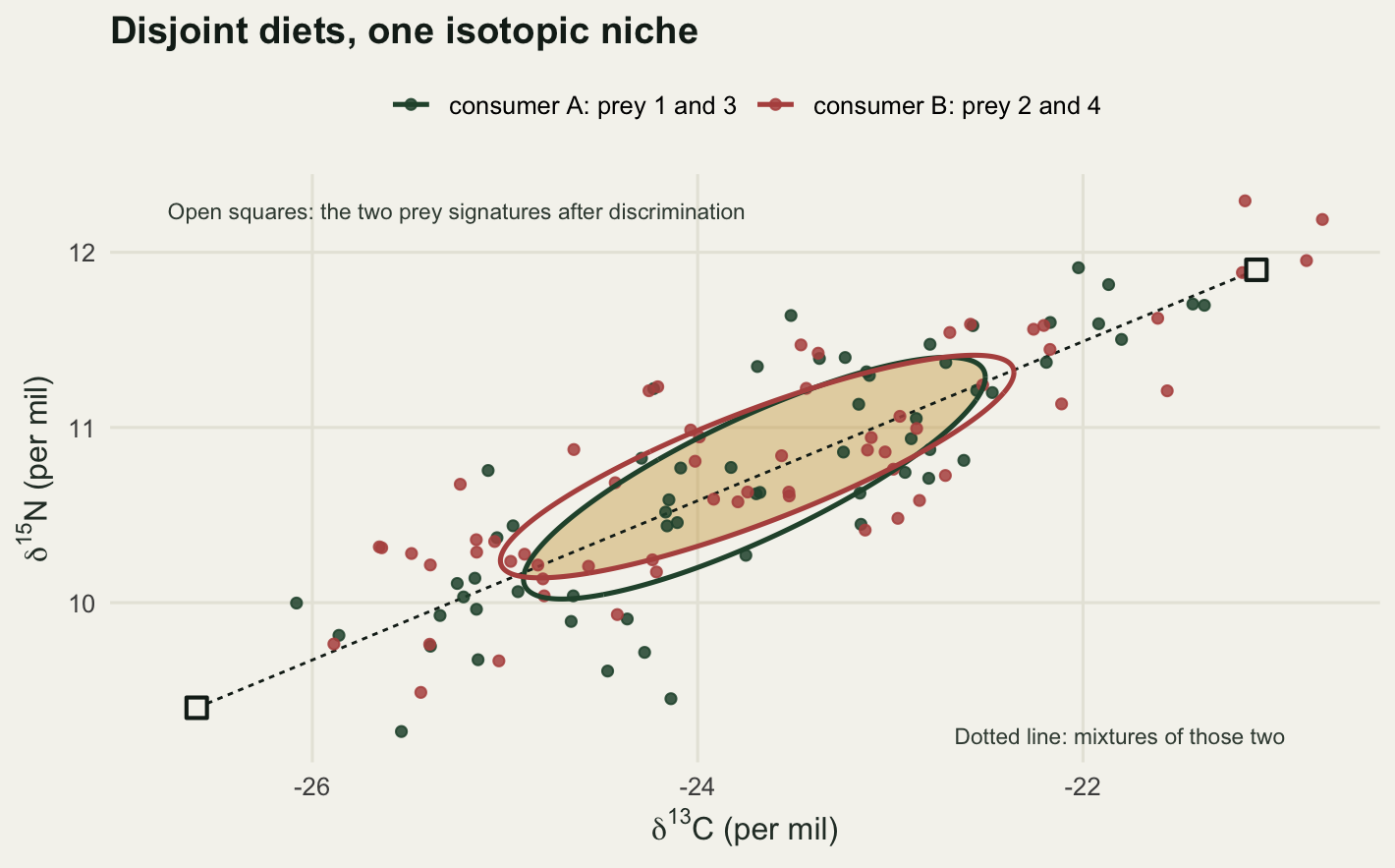
What to report instead
The post has measured four things that a single overlap percentage cannot carry, and they suggest a short reporting standard. Give both directional overlaps, since their ratio is the ratio of the two niche areas and readers can reconstruct it anyway. State the containment probability in the same sentence as the number, because the same pair of groups here moved from 0 to 0.4613 across a range of containments that are all in the published literature. Give an interval, not a point, because at 15 individuals per group the central 95 per cent of estimates spanned 0.8822 of the unit interval. And when the claim is about which group is narrower, report the posterior probability rather than the direction, because the direction alone is stated confidently and wrongly in 0.0983 of studies when the two groups are the same.
None of that rescues the measurement from the projection problem in the last section. It just stops the analysis from adding uncertainty of its own on top of it.
Where to go next
The natural next step is to stop treating the ellipse as the thing and start treating the diet as the thing, which means a mixing model that estimates prey proportions with their own uncertainty. That reintroduces the dimensions the isotope plane collapsed, at the cost of needing prey signatures and discrimination factors you can defend. The companion post on checking an isotopic niche analysis takes the diagnostics further, including what happens when the bivariate normal assumption behind every ellipse in this post is wrong.
References
Jackson AL, Inger R, Parnell AC, Bearhop S 2011 Journal of Animal Ecology 80(3):595-602 (10.1111/j.1365-2656.2011.01806.x)
Layman CA, Arrington DA, Montana CG, Post DM 2007 Ecology 88(1):42-48 (10.1890/0012-9658(2007)88[42:CSIRPF]2.0.CO;2)
Swanson HK, Lysy M, Power M, Stasko AD, Johnson JD, Reist JD 2015 Ecology 96(2):318-324 (10.1890/14-0235.1)
Newsome SD, Martinez del Rio C, Bearhop S, Phillips DL 2007 Frontiers in Ecology and the Environment 5(8):429-436 (10.1890/060150.1)
Anderson TW 2003 An Introduction to Multivariate Statistical Analysis. Wiley, ISBN 978-0-471-36091-9