library(ggplot2)
library(grid)

te_pal <- list(forest = "#275139", green = "#2f8f63", sage = "#93a87f",
               clay = "#b5534e", gold = "#cda23f", line = "#dad9ca",
               ink = "#16241d", paper = "#f5f4ee")

theme_te <- function() {
  theme_minimal(base_size = 12) +
    theme(panel.grid.minor = element_blank(),
          panel.grid.major = element_line(colour = "#e7e6dc"),
          plot.background = element_rect(fill = "#f5f4ee", colour = NA),
          panel.background = element_rect(fill = "#f5f4ee", colour = NA),
          plot.title = element_text(face = "bold", colour = te_pal$ink),
          axis.title = element_text(colour = "#2c3a31"))
}Checking an isotopic niche analysis
R
stable isotopes
trophic ecology
model diagnostics
ecology tutorial
ggplot2
Four checks for an isotopic niche analysis in R: sample size and power, the C:N lipid correction, a pipeline sweep, and tissue turnover in trophic ecology.
The three earlier posts of this cluster each hand back a number that goes straight into a results table. Isotopic niche width: hulls and ellipses returns a total area from the convex hull and a standard ellipse area corrected for sample size. Trophic position from stable isotopes returns a trophic position from a baseline, a consumer and a trophic discrimination factor. Isotopic niche overlap between groups returns the fraction of one ellipse that lies inside another. All three run on any two columns of numbers you give them, and all three print to four decimal places.
This post tries to break them. It is four checks, each a self-contained measurement against a truth that is known because we wrote it: how many individuals a niche width estimate needs before it means anything, and what a two-group comparison at that sample size can actually detect; what lipid does to the carbon axis and how much of that a C:N correction takes back; what happens when the same dataset is pushed through eight defensible versions of the same pipeline; and how much of a measured niche is really an artefact of which tissue was in the vial.
Nothing below is quoted from a rule of thumb. The thresholds, the critical values and the detectable effect sizes are all measured in the same simulator, because a number in a methods section is not a measurement. The simulator is a bivariate normal cloud in (\(\delta^{13}\)C, \(\delta^{15}\)N) space with a covariance matrix we choose, so the true standard ellipse area is available in closed form and every estimate can be scored against it.
The niche, and what counts as truth
A standard ellipse area is a function of the covariance matrix alone. For a bivariate cloud the area of the ellipse whose semi-axes are the square roots of the eigenvalues is \(\pi\) times the square root of the determinant, so if the covariance matrix is known the true SEA is known exactly. The sample version divides by \(n - 2\) rather than \(n - 1\) to remove the small-sample bias, and that is SEAc. The convex hull area has no such closed form and no such correction, which is the first hint of the trouble in check 3.
set.seed(20260718)

sea_from_S <- function(S) pi * sqrt(max(S[1, 1] * S[2, 2] - S[1, 2]^2, 0))

seac_xy <- function(x, y) {
  n <- length(x)
  sea_from_S(cov(cbind(x, y))) * (n - 1) / (n - 2)
}

hull_area <- function(x, y) {
  if (length(x) < 3) return(0)
  h <- chull(x, y)
  xs <- x[h]; ys <- y[h]
  abs(sum(xs * c(ys[-1], ys[1]) - c(xs[-1], xs[1]) * ys)) / 2
}

ellipse_pts <- function(x, y, p = 0.40, npt = 160) {
  ev <- eigen(cov(cbind(x, y)))
  ang <- seq(0, 2 * pi, length.out = npt)
  rad <- sqrt(qchisq(p, 2))
  z <- cbind(cos(ang), sin(ang)) %*% diag(sqrt(pmax(ev$values, 0))) %*% t(ev$vectors)
  data.frame(x = mean(x) + rad * z[, 1], y = mean(y) + rad * z[, 2])
}

sig_true <- matrix(c(0.90, 0.30, 0.30, 0.50), 2)
sea_true <- sea_from_S(sig_true)

round(c(sd_carbon = sqrt(sig_true[1, 1]), sd_nitrogen = sqrt(sig_true[2, 2]),
        correlation = sig_true[1, 2] / sqrt(sig_true[1, 1] * sig_true[2, 2]),
        true_SEA = sea_true,
        chisq_radius_at_40 = qchisq(0.40, 2),
        chisq_radius_at_95 = qchisq(0.95, 2)), 4)
sd_carbon sd_nitrogen correlation true_SEA
0.9487 0.7071 0.4472 1.8850
chisq_radius_at_40 chisq_radius_at_95
1.0217 5.9915 The population has a carbon standard deviation of 0.9487 and a nitrogen standard deviation of 0.7071 with a correlation of 0.4472, which is an unremarkable consumer group, and a true standard ellipse area of 1.885 squared permil. The two containment radii printed alongside are used in check 3: 1.0217 is the chi-squared quantile at 0.40, which is close enough to the standard ellipse that convention treats them as the same object, and 5.9915 is the quantile at 0.95.
Check 1: how many individuals does a niche width need?
Draw n individuals from that population, compute SEAc, and repeat. The estimate has no bias worth worrying about once the correction is applied, so the question is entirely about spread. We express it as the standard deviation of SEAc divided by the true area, because an ecologist reading a niche width wants to know how far off it might be as a fraction of itself.
sea_reps <- function(n, S, R) {
  z <- matrix(rnorm(2 * n * R), ncol = 2) %*% chol(S)
  x <- matrix(z[, 1], nrow = n); y <- matrix(z[, 2], nrow = n)
  cx <- x - rep(colMeans(x), each = n)
  cy <- y - rep(colMeans(y), each = n)
  s11 <- colSums(cx^2) / (n - 1)
  s22 <- colSums(cy^2) / (n - 1)
  s12 <- colSums(cx * cy) / (n - 1)
  pi * sqrt(pmax(s11 * s22 - s12^2, 0)) * (n - 1) / (n - 2)
}

n_grid <- c(5, 7, 10, 15, 20, 25, 30, 40, 50, 60, 80, 100, 125, 150, 200)
n_rep1 <- 4000

spread_tab <- do.call(rbind, lapply(n_grid, function(nn) {
  v <- sea_reps(nn, sig_true, n_rep1)
  data.frame(n = nn, rel_sd = sd(v) / sea_true, median_ratio = median(v) / sea_true,
             mean_ratio = mean(v) / sea_true)
}))
c(replicates_per_sample_size = n_rep1, largest_sample_size = max(n_grid))
replicates_per_sample_size largest_sample_size
4000 200 print(round(spread_tab, 4)) n rel_sd median_ratio mean_ratio
1 5 0.5731 0.8842 0.9931
2 7 0.4517 0.9443 1.0110
3 10 0.3513 0.9582 0.9963
4 15 0.2802 0.9837 1.0072
5 20 0.2352 0.9776 0.9984
6 25 0.2022 0.9839 0.9986
7 30 0.1871 0.9844 0.9975
8 40 0.1591 0.9951 1.0027
9 50 0.1451 0.9910 0.9969
10 60 0.1342 0.9944 1.0027
11 80 0.1134 0.9993 1.0025
12 100 0.1003 0.9960 0.9990
13 125 0.0904 0.9978 1.0029
14 150 0.0828 0.9976 1.0003
15 200 0.0705 0.9977 0.9973first_below <- function(thr) spread_tab$n[which(spread_tab$rel_sd < thr)[1]]
round(c(loose_threshold = 0.20, n_reaching_it = first_below(0.20),
tight_threshold = 0.10, n_reaching_it = first_below(0.10)), 3)loose_threshold n_reaching_it tight_threshold n_reaching_it
0.2 30.0 0.1 125.0 Across 4000 replicates at each sample size the mean of SEAc sits within about a per cent of the truth everywhere, so the correction does its job. The spread does not behave nearly as well. At five individuals the standard deviation of SEAc is 0.5731 of the true area, which means a niche width reported from five fish is routinely out by more than half. At ten it is 0.3513. The relative spread first falls below 0.20 at 30 individuals and below 0.10 at 125. The median ratio at five individuals is 0.8842, so half of all estimates from a group of five understate the truth by more than a tenth even though the mean is unbiased: the sampling distribution is right skewed, and the typical five-fish niche is too small while the occasional one is enormous.
That is precision. The currency that matters is a comparison, because almost nobody reports a niche width on its own. The question a study actually asks is whether group A has a wider niche than group B, so the honest sample size calculation is about the smallest true difference the comparison can find.
n_null <- 6000

crit_and_mdr <- function(nn) {
  d <- log(sea_reps(nn, sig_true, n_null)) - log(sea_reps(nn, sig_true, n_null))
  cc <- as.numeric(quantile(abs(d), 0.95))
  c(crit = cc, mdr = exp(cc - as.numeric(quantile(d, 0.20))))
}

pow_tab <- do.call(rbind, lapply(n_grid, function(nn) data.frame(n = nn, t(crit_and_mdr(nn)))))
c(null_replicates = n_null)
null_replicates
6000 print(round(pow_tab, 4)) n crit mdr
1 5 1.7490 12.1328
2 7 1.2859 6.2031
3 10 1.0124 4.2403
4 15 0.7680 2.9787
5 20 0.6782 2.6405
6 25 0.5871 2.3208
7 30 0.5257 2.1171
8 40 0.4506 1.9037
9 50 0.3962 1.7641
10 60 0.3662 1.6773
11 80 0.3118 1.5619
12 100 0.2857 1.5031
13 125 0.2502 1.4278
14 150 0.2275 1.3847
15 200 0.1942 1.3247nv <- 25
cv <- pow_tab[pow_tab$n == nv, ]
check_a <- sea_reps(nv, sig_true, n_null)
check_b <- sea_reps(nv, cv$mdr * sig_true, n_null)
round(c(detectable_ratio_n10 = pow_tab$mdr[pow_tab$n == 10],
detectable_ratio_n25 = cv$mdr,
detectable_ratio_n60 = pow_tab$mdr[pow_tab$n == 60],
detectable_ratio_n200 = pow_tab$mdr[pow_tab$n == 200],
realised_power_at_n25 = mean(abs(log(check_b) - log(check_a)) > cv$crit)), 4) detectable_ratio_n10 detectable_ratio_n25 detectable_ratio_n60
4.2403 2.3208 1.6773
detectable_ratio_n200 realised_power_at_n25
1.3247 0.8043 The test statistic is the log ratio of the two SEAc values. Its null distribution depends on sample size and on nothing else, because scaling a covariance matrix scales the ellipse area by the same factor and the ratio does not care about the units. That makes the calculation exact rather than approximate: the alternative distribution is the null shifted by the log of the true ratio, so the smallest detectable ratio is the 95th percentile of the absolute null statistic minus the 20th percentile of the signed one, exponentiated. The last line confirms it by brute force, simulating at that ratio and getting a rejection rate of 0.8043.
The numbers are unkind. At ten individuals per group the two-group comparison detects a true difference of 4.2403 fold and nothing smaller. At 25 per group it detects 2.3208 fold. At 60 per group, which is a serious sampling effort in most systems, it detects 1.6773 fold. Even at 200 per group the smallest detectable difference is 1.3247 fold. A study that samples 25 of each of two groups and reports no significant difference in niche width has found out that the niches do not differ by more than a factor of two and a bit, which is usually not the question that was asked.
panel_levels <- c("Relative standard deviation of SEAc",
                  "Smallest ratio found with 80 per cent power")
f1 <- rbind(
  data.frame(n = spread_tab$n, value = spread_tab$rel_sd, panel = panel_levels[1]),
  data.frame(n = pow_tab$n, value = pow_tab$mdr, panel = panel_levels[2]))
f1$panel <- factor(f1$panel, levels = panel_levels)
rules <- data.frame(yv = c(0.20, 0.10, 1),
                    panel = factor(panel_levels[c(1, 1, 2)], levels = panel_levels))
marks <- data.frame(n = c(10, 25, 60),
                    value = pow_tab$mdr[match(c(10, 25, 60), pow_tab$n)],
                    panel = factor(panel_levels[2], levels = panel_levels))

ggplot(f1, aes(n, value)) +
  geom_hline(data = rules, aes(yintercept = yv), colour = te_pal$clay,
             linetype = "22", linewidth = 0.6) +
  geom_line(colour = te_pal$forest, linewidth = 0.9) +
  geom_point(colour = te_pal$green, size = 1.8) +
  geom_point(data = marks, colour = te_pal$clay, size = 3.4) +
  facet_wrap(~panel, scales = "free_y") +
  scale_x_log10(breaks = c(5, 10, 25, 60, 150)) +
  labs(x = "Individuals per group", y = NULL,
       title = "What a niche width costs in animals") +
  theme_te() +
  theme(strip.text = element_text(colour = te_pal$ink, face = "bold"))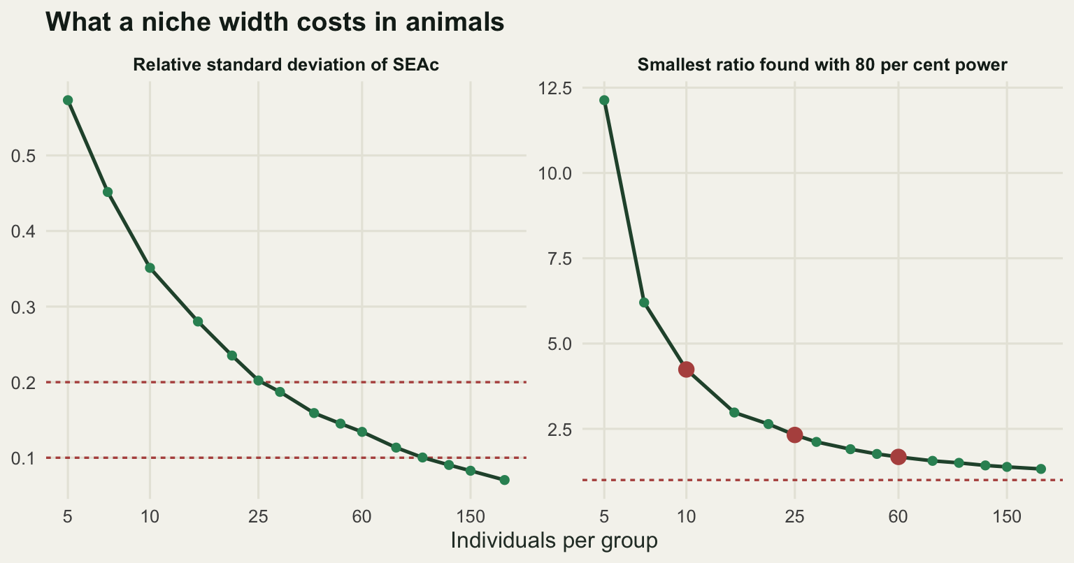
Check 2: lipids, and what the C:N correction leaves behind
Lipid is depleted in \(\delta^{13}\)C relative to protein, so a fat individual sits artificially low on the carbon axis for reasons that have nothing to do with what it ate. The simulator makes that explicit. Each individual has a lipid-free carbon and nitrogen value drawn from the population above, plus a lipid fraction of its carbon that rises with body size. Nitrogen only comes from the protein pool, so the bulk C:N ratio is the lipid-free ratio divided by one minus the lipid fraction, and the bulk carbon value is the lipid-free value pulled down in proportion to the lipid fraction.
The correction applied is the linear equation in C:N that most studies use, which adds \(0.99 \times \mathrm{C{:}N} - 3.32\) to the measured value. It is calibrated on real tissue, not on our two-pool bookkeeping, so it is worth asking first what lipid offset the equation implies at each C:N. That is a one-line inversion.
cn_prot <- 3.35
delta_lip <- 6.5
post_norm <- function(dC, cn) dC - 3.32 + 0.99 * cn
implied_offset <- function(cn) (0.99 * cn - 3.32) / (1 - cn_prot / cn)

sim_lipid <- function(n, muC, muN, S, lip_mean, lip_sd, cn_err = 0.06) {
  z <- matrix(rnorm(2 * n), ncol = 2) %*% chol(S)
  size <- rnorm(n)
  pl <- pmin(pmax(lip_mean + lip_sd * (0.8 * size + 0.6 * rnorm(n)), 0.03), 0.55)
  cn <- cn_prot / (1 - pl) + rnorm(n, 0, cn_err)
  out <- data.frame(size = size, lipid = pl, cn = cn,
                    lfC = muC + z[, 1], N = muN + z[, 2],
                    bulkC = muC + z[, 1] - delta_lip * pl)
  out$corrC <- post_norm(out$bulkC, out$cn)
  out
}

n2 <- 120
g2 <- sim_lipid(n2, -24, 8.5, sig_true, 0.20, 0.13)
round(c(lipid_free_CN = cn_prot, true_lipid_offset = delta_lip, individuals = n2,
        correction_slope = 0.99, correction_intercept = -3.32,
        cor_size_lipid = cor(g2$size, g2$lipid),
        min_CN = min(g2$cn), max_CN = max(g2$cn),
        implied_offset_at_CN_4 = implied_offset(4),
        implied_offset_at_CN_7 = implied_offset(7)), 4)
lipid_free_CN true_lipid_offset individuals
3.3500 6.5000 120.0000
correction_slope correction_intercept cor_size_lipid
0.9900 -3.3200 0.7980
min_CN max_CN implied_offset_at_CN_4
3.3569 5.9841 3.9385
implied_offset_at_CN_7
6.9233 s_lf <- seac_xy(g2$lfC, g2$N)
s_bulk <- seac_xy(g2$bulkC, g2$N)
s_corr <- seac_xy(g2$corrC, g2$N)
round(c(centroid_shift_bulk = mean(g2$bulkC) - mean(g2$lfC),
centroid_shift_corrected = mean(g2$corrC) - mean(g2$lfC),
shift_removed_percent = 100 * (1 - (mean(g2$corrC) - mean(g2$lfC)) /
(mean(g2$bulkC) - mean(g2$lfC))),
SEAc_truth = s_lf, SEAc_bulk = s_bulk, SEAc_corrected = s_corr,
inflation_percent = 100 * (s_bulk / s_lf - 1),
residual_inflation_percent = 100 * (s_corr / s_lf - 1)), 4) centroid_shift_bulk centroid_shift_corrected
-1.2004 -0.3705
shift_removed_percent SEAc_truth
69.1327 1.7573
SEAc_bulk SEAc_corrected
2.3318 1.7999
inflation_percent residual_inflation_percent
32.6875 2.4247 The group has a C:N running from 3.3569 to 5.9841, which is a normal range for muscle in a species that stores fat, and the lipid fraction correlates with size at 0.798. Lipid drags the group centroid down the carbon axis by 1.2004 permil. It also inflates the niche: SEAc rises from 1.7573 to 2.3318, an inflation of 32.6875 per cent, purely because condition varies among individuals and condition moves carbon.
The correction removes 69.13 per cent of the centroid shift, leaving 0.3705 permil, and it removes almost all of the area inflation, leaving 2.4247 per cent. That asymmetry is worth pausing on. The residual on the area is small because area depends on the square of the residual amplitude, so knocking two thirds off the lipid signal knocks about nine tenths off its contribution to the variance. The residual on the centroid is not small, and a centroid is what a niche position comparison uses.
Why two thirds and not all of it? The two implied offsets say it. The linear equation supplies a correction consistent with a lipid to protein offset of 3.9385 permil at a C:N of 4 and 6.9233 permil at a C:N of 7. It cannot be consistent with a single offset at both, because mass balance makes the required correction a curve in C:N and the equation is a straight line through it. Our simulator uses a fixed offset of 6.5 permil, and the equation implies a different one at each C:N: at the fattest individual here it implies 5.9163 permil, and the implied offset falls as C:N falls. A reader is entitled to say that this makes the residual a property of our bookkeeping rather than of the equation. That is exactly the point: the equation was fitted across taxa and tissues, and the offset in your animal is not the offset it was fitted to.
Now the part that changes conclusions. Take two groups whose lipid-free isotopes are drawn from the same distribution, so their diets are identical by construction, and give one of them a mean lipid fraction of 0.08 and the other 0.28.
gA <- sim_lipid(n2, -24, 8.5, sig_true, 0.08, 0.04)
gB <- sim_lipid(n2, -24, 8.5, sig_true, 0.28, 0.07)
gap <- function(v, w) mean(v) - mean(w)
round(c(mean_lipid_lean = mean(gA$lipid), mean_lipid_rich = mean(gB$lipid),
        true_carbon_gap = gap(gA$lfC, gB$lfC),
        bulk_carbon_gap = gap(gA$bulkC, gB$bulkC),
        corrected_carbon_gap = gap(gA$corrC, gB$corrC),
        bulk_gap_in_sd = gap(gA$bulkC, gB$bulkC) / sqrt(sig_true[1, 1]),
        corrected_gap_in_sd = gap(gA$corrC, gB$corrC) / sqrt(sig_true[1, 1])), 4)
mean_lipid_lean mean_lipid_rich true_carbon_gap
0.0812 0.2839 0.0671
bulk_carbon_gap corrected_carbon_gap bulk_gap_in_sd
1.3852 0.3298 1.4602
corrected_gap_in_sd
0.3477 The true separation on the carbon axis is 0.0671 permil, which is sampling noise around zero. The bulk data show a separation of 1.3852 permil, which is 1.4602 within-group standard deviations, a gap any reader would describe as a clear difference in carbon source. There is no difference in carbon source. There is a difference in body condition. After correction the gap falls to 0.3298 permil, or 0.3477 standard deviations, which is smaller but still in the direction that condition put it.
view_levels <- c("Bulk values", "After the C:N correction", "Lipid free truth")
grp_levels <- c("Lean group", "Lipid rich group")
pack <- function(cA, cB, lab) rbind(
  data.frame(C = cA, N = gA$N, group = grp_levels[1], view = lab),
  data.frame(C = cB, N = gB$N, group = grp_levels[2], view = lab))
pts2 <- rbind(pack(gA$bulkC, gB$bulkC, view_levels[1]),
              pack(gA$corrC, gB$corrC, view_levels[2]),
              pack(gA$lfC, gB$lfC, view_levels[3]))
pts2$view <- factor(pts2$view, levels = view_levels)
pts2$group <- factor(pts2$group, levels = grp_levels)
ell2 <- do.call(rbind, lapply(split(pts2, list(pts2$group, pts2$view)), function(z)
  data.frame(ellipse_pts(z$C, z$N), group = z$group[1], view = z$view[1])))

ggplot(pts2, aes(C, N, colour = group)) +
  geom_point(size = 1.1, alpha = 0.7) +
  geom_path(data = ell2, aes(x, y, colour = group), linewidth = 0.9) +
  facet_wrap(~view) +
  scale_colour_manual(values = c(te_pal$forest, te_pal$clay), name = NULL) +
  labs(x = "Carbon, permil", y = "Nitrogen, permil",
       title = "One diet, three versions of the picture") +
  theme_te() +
  theme(legend.position = "top",
        strip.text = element_text(colour = te_pal$ink, face = "bold"))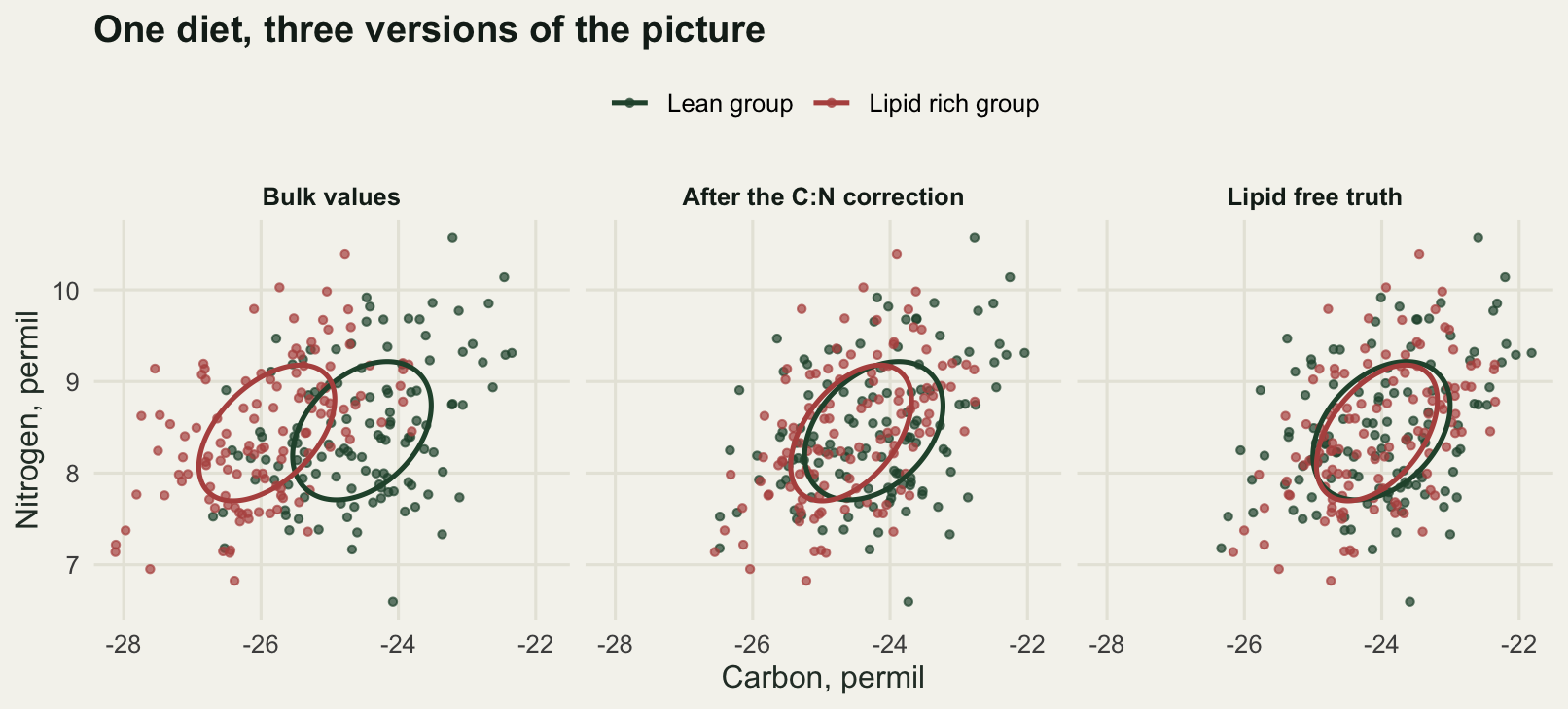
Check 3: the pipeline, not the last step
An isotopic niche result is not one calculation. It is a chain: decide whether to lipid correct, decide whether the width is a hull or an ellipse, decide what fraction of the population the region is meant to contain, then compare. Checking the last link tells you nothing about the chain. So take one simulated dataset and run all eight combinations of three binary decisions through to a published sentence.
Group A truly has the wider niche, by a factor of 1.8. Group B is the lipid-rich one, which is the situation that arises whenever the groups differ in condition: a spawning population against a post-spawning one, an inshore group against an offshore one, adults against juveniles. The containment probability is either 0.40, the conventional standard ellipse, or 0.95. For the ellipse the containment is a multiplier on the area; for the hull we take the convex hull of the individuals inside the corresponding Mahalanobis contour, which is the hull peeling that a containment choice implies.
n3 <- 110
S_B <- matrix(c(0.25, 0.08, 0.08, 0.16), 2)
ratio_true <- 1.8
S_A <- ratio_true * S_B

set.seed(414)
dA <- sim_lipid(n3, -24.5, 8.8, S_A, 0.06, 0.03)
dB <- sim_lipid(n3, -24.5, 8.8, S_B, 0.26, 0.18)

round(c(per_group = n3, true_SEA_A = sea_from_S(S_A), true_SEA_B = sea_from_S(S_B),
        true_ratio = ratio_true,
        mean_lipid_A = mean(dA$lipid), mean_lipid_B = mean(dB$lipid),
        max_CN_A = max(dA$cn), max_CN_B = max(dB$cn)), 4)
per_group true_SEA_A true_SEA_B true_ratio mean_lipid_A mean_lipid_B
110.0000 1.0366 0.5759 1.8000 0.0648 0.2940
max_CN_A max_CN_B
3.9926 7.5268 round(c(SEAc_lipid_free_A = seac_xy(dA$lfC, dA$N), SEAc_lipid_free_B = seac_xy(dB$lfC, dB$N),
SEAc_bulk_A = seac_xy(dA$bulkC, dA$N), SEAc_bulk_B = seac_xy(dB$bulkC, dB$N),
SEAc_corrected_A = seac_xy(dA$corrC, dA$N),
SEAc_corrected_B = seac_xy(dB$corrC, dB$N),
residual_inflation_B = seac_xy(dB$corrC, dB$N) / seac_xy(dB$lfC, dB$N)), 4) SEAc_lipid_free_A SEAc_lipid_free_B SEAc_bulk_A
1.0232 0.5795 1.0959
SEAc_bulk_B SEAc_corrected_A SEAc_corrected_B
1.4151 1.0463 0.7061
residual_inflation_B
1.2184 The lipid-free areas are 1.0232 and 0.5795, a ratio in the region of the 1.8 we built in. In bulk values group B measures 1.4151 against group A’s 1.0959, so the narrower group now looks like the wider one. Correction takes group B down to 0.7061, which is still 1.2184 times its true area, because the residual left in check 2 is largest in exactly the group whose C:N spans the widest range, here up to 7.5268.
width_metric <- function(x, y, metric, p) {
  n <- length(x)
  S <- cov(cbind(x, y))
  if (metric == "ellipse")
    return(pi * qchisq(p, 2) * sqrt(max(S[1, 1] * S[2, 2] - S[1, 2]^2, 0)) * (n - 1) / (n - 2))
  md <- mahalanobis(cbind(x, y), c(mean(x), mean(y)), S)
  keep <- md <= qchisq(p, 2)
  if (sum(keep) < 3) return(NA_real_)
  hull_area(x[keep], y[keep])
}

n_boot <- 500
run_pipeline <- function(metric, p, corrected) {
  xa <- if (corrected) dA$corrC else dA$bulkC
  xb <- if (corrected) dB$corrC else dB$bulkC
  obs <- log(width_metric(xa, dA$N, metric, p) / width_metric(xb, dB$N, metric, p))
  set.seed(9001)
  bs <- replicate(n_boot, {
    ia <- sample.int(n3, n3, TRUE); ib <- sample.int(n3, n3, TRUE)
    log(width_metric(xa[ia], dA$N[ia], metric, p) /
          width_metric(xb[ib], dB$N[ib], metric, p))
  })
  ci <- quantile(bs, c(0.025, 0.975), na.rm = TRUE)
  data.frame(lipid = ifelse(corrected, "corrected", "bulk"), metric = metric,
             containment = p, ratio = exp(obs), lo = exp(ci[1]), hi = exp(ci[2]),
             verdict = if (ci[1] > 0) "A wider than B" else
               if (ci[2] < 0) "B wider than A" else
                 "no difference at the 95 per cent level")
}

grid3 <- expand.grid(p = c(0.40, 0.95), metric = c("ellipse", "hull"),
                     corrected = c(FALSE, TRUE), stringsAsFactors = FALSE)
tab3 <- do.call(rbind, lapply(seq_len(nrow(grid3)), function(i)
  run_pipeline(grid3$metric[i], grid3$p[i], grid3$corrected[i])))
c(bootstrap_resamples = n_boot, pipelines = nrow(tab3))
bootstrap_resamples pipelines
500 8 print(cbind(tab3[, 1:3], round(tab3[, 4:6], 4), verdict = tab3$verdict), row.names = FALSE) lipid metric containment ratio lo hi
bulk ellipse 0.40 0.7744 0.6210 0.9770
bulk ellipse 0.95 0.7744 0.6210 0.9770
bulk hull 0.40 0.6930 0.4975 1.2274
bulk hull 0.95 0.8105 0.5974 0.9811
corrected ellipse 0.40 1.4818 1.1589 1.8807
corrected ellipse 0.95 1.4818 1.1589 1.8807
corrected hull 0.40 1.7145 0.9717 2.4226
corrected hull 0.95 1.6331 1.1380 2.1069
verdict
B wider than A
B wider than A
no difference at the 95 per cent level
B wider than A
A wider than B
A wider than B
no difference at the 95 per cent level
A wider than Bc(distinct_verdicts = length(unique(tab3$verdict)))distinct_verdicts
3 Eight pipelines, one dataset, three verdicts on this run. Three of them report that group B has the wider niche, three report that group A does, and two report no difference at the 95 per cent level. Group A is the wider one, so three pipelines have the direction exactly backwards and are confident about it. Half the intervals in the table exclude the true ratio of 1.8 altogether, and none of the eight point estimates reaches it: the best of them, the corrected hull at a containment of 0.40, returns 1.7145, and the corrected ellipse returns 1.4818.
The decision that flips the sign is the lipid one. Every bulk pipeline points one way and every corrected pipeline points the other, and lipid correction is the decision most often disposed of in a single clause of a methods section. The decision that does nothing at all is the containment probability, and the four ellipse rows show why: they pair up within each lipid decision, identical to four decimal places in the point estimate and in both interval limits, because the containment enters an ellipse area as a constant multiplier that cancels in a ratio. It cancels in the ratio, it cancels in the bootstrap, and it changes only the number printed in the table. For the hull it does not cancel, because peeling to a 0.40 contour throws away three fifths of the individuals; that pipeline returns a different estimate from the same hull at 0.95, on a wider interval.
tab3$label <- sprintf("%s, %s, p = %.2f", tab3$lipid, tab3$metric, tab3$containment)
tab3$label <- factor(tab3$label, levels = tab3$label[order(tab3$ratio)])

ggplot(tab3, aes(ratio, label, colour = verdict)) +
  geom_vline(xintercept = 1, colour = te_pal$ink, linewidth = 0.6) +
  geom_vline(xintercept = ratio_true, colour = te_pal$gold,
             linetype = "22", linewidth = 0.8) +
  geom_errorbar(aes(xmin = lo, xmax = hi), orientation = "y", width = 0.25, linewidth = 0.8) +
  geom_point(size = 3) +
  scale_x_log10(breaks = c(0.5, 0.75, 1, 1.5, 2, 2.5)) +
  scale_colour_manual(values = c("A wider than B" = te_pal$forest,
                                 "B wider than A" = te_pal$clay,
                                 "no difference at the 95 per cent level" = te_pal$gold),
                      name = NULL) +
  guides(colour = guide_legend(nrow = 3)) +
  labs(x = "Estimated niche width, group A over group B", y = NULL,
       title = "Eight defensible pipelines, three answers") +
  theme_te() +
  theme(legend.position = "top", legend.text = element_text(size = 9))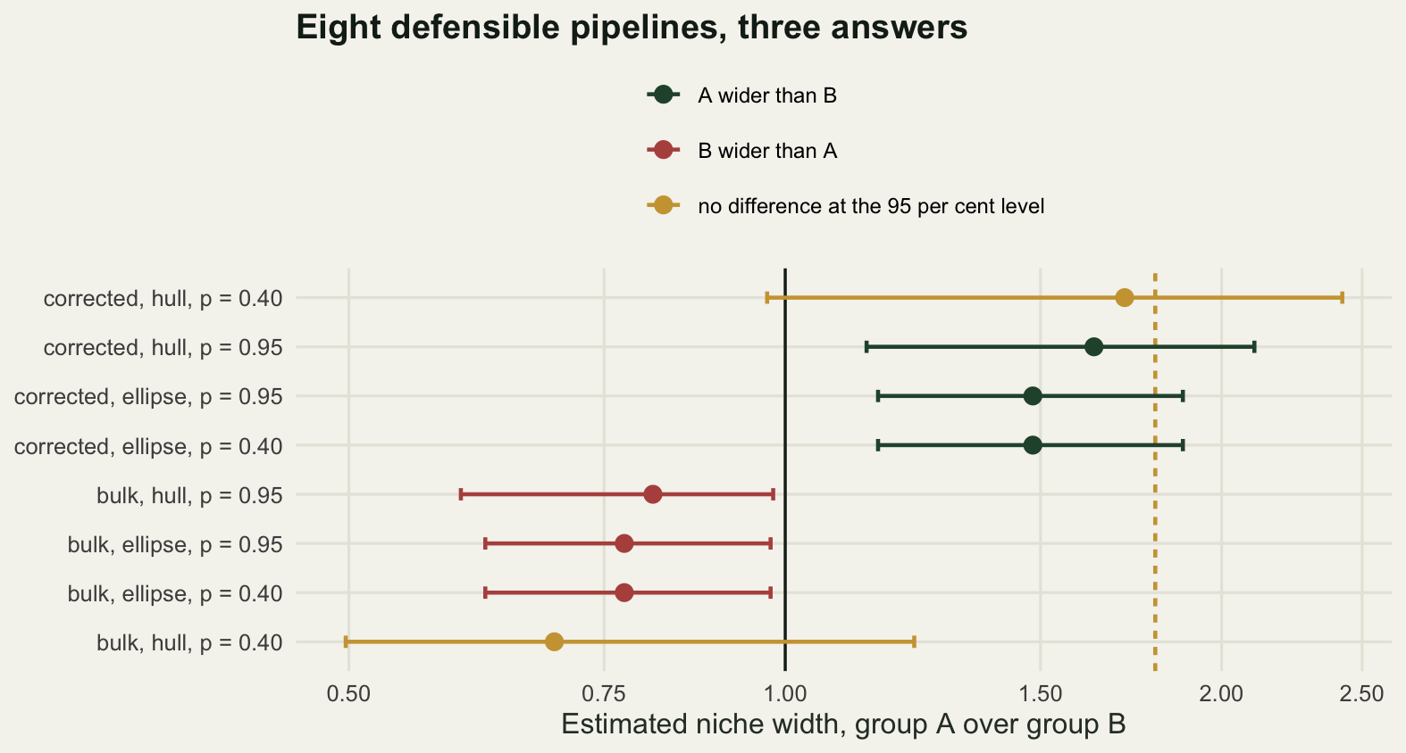
Check 4: two tissues, two windows, one animal
Blood plasma turns over in days and muscle in months, so the two tissues of the same animal are averaging its diet over different windows. Model the tissue value as an exponentially weighted average of past diet with a rate set by the tissue half-life. For a diet that varies sinusoidally through the year this has a closed form: the tissue keeps the same period, its amplitude is damped by one over the square root of one plus the ratio of the seasonal frequency to the turnover rate squared, and it lags the diet by the arctangent of that same ratio.
hl_fast <- 5; hl_slow <- 90
wfreq <- 2 * pi / 365
lam_of <- function(hl) log(2) / hl
damp_of <- function(hl) 1 / sqrt(1 + (wfreq / lam_of(hl))^2)
lag_of <- function(hl) atan(wfreq / lam_of(hl))

muC4 <- -23.5; muN4 <- 9.2; aC4 <- 2.2; aN4 <- 1.6
phiC <- 0; phiN <- pi / 3
sd_ind <- 0.45; sd_meas <- 0.15
tdf_n <- 3.4; base_n <- 4.6; base_tl <- 2
n4 <- 60

tissue_vals <- function(hl, tt, ic, inn) {
  kk <- damp_of(hl); lg <- lag_of(hl)
  data.frame(C = muC4 + kk * aC4 * sin(wfreq * tt + phiC - lg) + ic +
               rnorm(length(tt), 0, sd_meas),
             N = muN4 + kk * aN4 * sin(wfreq * tt + phiN - lg) + inn +
               rnorm(length(tt), 0, sd_meas))
}

set.seed(707)
tt <- runif(n4, 0, 365)
ic <- rnorm(n4, 0, sd_ind); inn <- rnorm(n4, 0, sd_ind)
plasma <- tissue_vals(hl_fast, tt, ic, inn)
muscle <- tissue_vals(hl_slow, tt, ic, inn)
sp <- seac_xy(plasma$C, plasma$N); sm <- seac_xy(muscle$C, muscle$N)

round(c(fast_half_life_days = hl_fast, slow_half_life_days = hl_slow,
        fast_damping = damp_of(hl_fast), slow_damping = damp_of(hl_slow),
        fast_lag_days = lag_of(hl_fast) / wfreq,
        slow_lag_days = lag_of(hl_slow) / wfreq), 4)
fast_half_life_days slow_half_life_days fast_damping slow_damping
5.0000 90.0000 0.9924 0.4084
fast_lag_days slow_lag_days
7.1767 66.8115 round(c(individuals = n4, SEAc_plasma = sp, SEAc_muscle = sm, ratio = sp / sm), 4)individuals SEAc_plasma SEAc_muscle ratio
60.0000 6.3358 1.6658 3.8035 day <- 0:364
tp_of <- function(hl) base_tl + (muN4 + damp_of(hl) * aN4 *
sin(wfreq * day + phiN - lag_of(hl)) - base_n) / tdf_n
tp_gap <- tp_of(hl_fast) - tp_of(hl_slow)
round(c(discrimination_factor = tdf_n, max_TP_gap = max(abs(tp_gap)),
day_of_max_gap = day[which.max(abs(tp_gap))],
annual_mean_gap = mean(tp_gap)), 4)discrimination_factor max_TP_gap day_of_max_gap
3.4000 0.4026 13.0000
annual_mean_gap
0.0000 A plasma half-life of five days gives a damping of 0.9924 and a lag of 7.1767 days, so plasma tracks the seasonal diet almost exactly. A muscle half-life of 90 days gives a damping of 0.4084 and a lag of 66.8115 days, so muscle sees a signal less than half the size and two months behind.
Sixty animals sampled at random through the year give a plasma SEAc of 6.3358 and a muscle SEAc of 1.6658 for the same sixty animals. The ratio is 3.8035. The animals are identical, the diet is identical, and the individual variation is identical; the only thing that differs is which vial went into the mass spectrometer. Most of the plasma niche is seasonal variation in the diet that muscle has already averaged away.
Trophic position behaves differently, and the difference is instructive. Averaged over the year the two tissues give the same trophic position, to machine precision, because the exponential weighting is unbiased for a stationary diet. But a field season is not a year. The largest gap between the plasma trophic position and the muscle trophic position is 0.4026 of a trophic level, on day 13 of the cycle, which is where the fast tissue is already high on the seasonal rise while the slow tissue, damped and two months behind, is still passing through its annual mean. A study that samples once, as almost all studies do, gets whichever point on that curve its field season happened to fall on.
crit60 <- unlist(pow_tab[pow_tab$n == n4, c("crit", "mdr")])
nfd <- 400
set.seed(808)
induced <- replicate(nfd, {
  a <- tissue_vals(hl_fast, runif(n4, 0, 365), rnorm(n4, 0, sd_ind), rnorm(n4, 0, sd_ind))
  b <- tissue_vals(hl_slow, runif(n4, 0, 365), rnorm(n4, 0, sd_ind), rnorm(n4, 0, sd_ind))
  log(seac_xy(a$C, a$N) / seac_xy(b$C, b$N))
})
round(c(replicates = nfd, critical_value = crit60["crit"],
        detectable_ratio = crit60["mdr"],
        median_induced_ratio = exp(median(induced)),
        significant_fraction = mean(abs(induced) > crit60["crit"])), 4)
replicates critical_value.crit detectable_ratio.mdr
400.0000 0.3662 1.6773
median_induced_ratio significant_fraction
3.4714 1.0000 Now put that inside a comparison. Group A is sampled by plasma and group B by muscle, both groups eat exactly the same thing, and both are sampled through the year at 60 individuals each. Across 400 such studies the median apparent ratio of niche widths is 3.4714, against a truth of one. The critical value from check 1 at 60 per group is 0.3662 on the log scale, corresponding to a detectable ratio of 1.6773, and the induced difference clears it in every single one of the 400 replicates. A mixed-tissue design does not merely add noise. It manufactures a large, highly significant difference in niche width where none exists, and it does so reliably enough that no amount of replication will save you.
curve_levels <- c("Diet", "Plasma", "Muscle")
curves <- rbind(
  data.frame(day = day, value = muN4 + aN4 * sin(wfreq * day + phiN), series = curve_levels[1]),
  data.frame(day = day, value = muN4 + damp_of(hl_fast) * aN4 *
               sin(wfreq * day + phiN - lag_of(hl_fast)), series = curve_levels[2]),
  data.frame(day = day, value = muN4 + damp_of(hl_slow) * aN4 *
               sin(wfreq * day + phiN - lag_of(hl_slow)), series = curve_levels[3]))
curves$series <- factor(curves$series, levels = curve_levels)

p_left <- ggplot(curves, aes(day, value, colour = series, linetype = series)) +
  geom_vline(xintercept = day[which.max(abs(tp_gap))], colour = "#8a8977",
             linetype = "12", linewidth = 0.7) +
  geom_line(linewidth = 0.9) +
  annotate("text", x = 22, y = muN4 + aN4 + 0.62, hjust = 0, size = 2.9,
           colour = "#57564a",
           label = "Vertical line: the day the tissues differ most") +
  scale_colour_manual(values = c("#243318", te_pal$green, te_pal$clay), name = NULL) +
  scale_linetype_manual(values = c("42", "solid", "solid"), name = NULL) +
  labs(x = "Day of year", y = "Nitrogen, permil",
       title = "Two tissues, two windows") +
  theme_te() +
  theme(legend.position = "top")

tis_levels <- c("Plasma", "Muscle")
pts4 <- rbind(data.frame(plasma, tissue = tis_levels[1]),
              data.frame(muscle, tissue = tis_levels[2]))
pts4$tissue <- factor(pts4$tissue, levels = tis_levels)
ell4 <- rbind(data.frame(ellipse_pts(plasma$C, plasma$N), tissue = tis_levels[1]),
              data.frame(ellipse_pts(muscle$C, muscle$N), tissue = tis_levels[2]))
ell4$tissue <- factor(ell4$tissue, levels = tis_levels)

p_right <- ggplot(pts4, aes(C, N, colour = tissue)) +
  geom_point(size = 1.4, alpha = 0.8) +
  geom_path(data = ell4, aes(x, y, colour = tissue), linewidth = 0.9) +
  scale_colour_manual(values = c(te_pal$green, te_pal$clay), name = NULL) +
  labs(x = "Carbon, permil", y = "Nitrogen, permil",
       title = "The same sixty animals") +
  theme_te() +
  theme(legend.position = "top")

grid.newpage()
pushViewport(viewport(layout = grid.layout(1, 2)))
print(p_left, vp = viewport(layout.pos.row = 1, layout.pos.col = 1))
print(p_right, vp = viewport(layout.pos.row = 1, layout.pos.col = 2))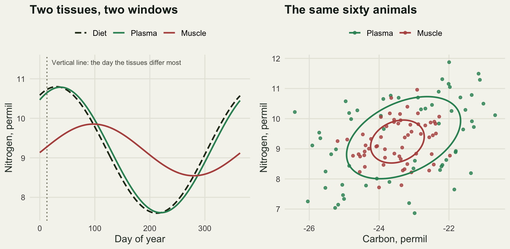
What none of these checks can see
Every check above is internal. Each one compares an isotopic estimate against the isotopic truth that generated it, and every one of them can pass while the ecology is read backwards. The boundary has two sides and both are measurable.
On the first side, two groups can be isotopically identical and eat nothing in common. Build two consumers, each mixing two sources, with no source shared between them, and choose the second pair so that its mixing line runs parallel to the first through the same midpoint. The two groups are then the same bivariate cloud.
A1 <- c(-28, 5); A2 <- c(-20, 11)
B1 <- c(-27, 5.75); B2 <- c(-21, 10.25)
nh <- 200
sd_pA <- 0.09
sd_pB <- sd_pA * (A2[1] - A1[1]) / (B2[1] - B1[1])

mix_group <- function(s1, s2, sdp, n) {
  pr <- rnorm(n, 0.5, sdp)
  cbind(s1[1] + pr * (s2[1] - s1[1]) + rnorm(n, 0, 0.25),
        s1[2] + pr * (s2[2] - s1[2]) + rnorm(n, 0, 0.25))
}

ell_overlap <- function(pa, pb, nmc = 40000) {
  ea <- eigen(cov(pa))
  ang <- runif(nmc, 0, 2 * pi); rad <- sqrt(runif(nmc))
  z <- cbind(rad * cos(ang), rad * sin(ang)) %*% diag(sqrt(ea$values)) %*% t(ea$vectors)
  mean(mahalanobis(cbind(z[, 1] + mean(pa[, 1]), z[, 2] + mean(pa[, 2])),
                   colMeans(pb), cov(pb)) <= 1)
}

set.seed(99)
ha <- mix_group(A1, A2, sd_pA, nh)
hb <- mix_group(B1, B2, sd_pB, nh)
hc <- mix_group(A1 + c(1.2, 0.8), A2 + c(1.2, 0.8), sd_pA, nh)

round(c(individuals_per_group = nh, shared_sources = 0,
        centroid_distance = sqrt(sum((colMeans(ha) - colMeans(hb))^2)),
        SEAc_ratio = seac_xy(ha[, 1], ha[, 2]) / seac_xy(hb[, 1], hb[, 2]),
        ellipse_overlap = ell_overlap(ha, hb)), 4)
individuals_per_group shared_sources centroid_distance
200.0000 0.0000 0.1607
SEAc_ratio ellipse_overlap
1.0068 0.8860 round(c(baseline_shift_carbon = 1.2, baseline_shift_nitrogen = 0.8,
shifted_centroid_distance = sqrt(sum((colMeans(ha) - colMeans(hc))^2)),
shifted_SEAc_ratio = seac_xy(ha[, 1], ha[, 2]) / seac_xy(hc[, 1], hc[, 2]),
shifted_overlap = ell_overlap(ha, hc)), 4) baseline_shift_carbon baseline_shift_nitrogen shifted_centroid_distance
1.2000 0.8000 1.4867
shifted_SEAc_ratio shifted_overlap
1.0211 0.0874 The two groups share no prey at all. Their centroids are 0.1607 permil apart, their SEAc values differ by a factor of 1.0068, and 0.8860 of the first group’s standard ellipse lies inside the second. Sample size, lipid content, metric choice and tissue are all clean here; every check in this post passes on both groups; and the conclusion an isotopic niche analysis supports, that these two consumers occupy the same trophic niche, is false. This is the same degeneracy the overlap post ran into from the other direction, where two consumers with completely disjoint diets returned an overlap indistinguishable from one, and it is a property of the data type rather than of the estimator.
The other side is the same problem inverted. Build a third group that mixes the first group’s two sources in the same proportions on average, but with both sources displaced by 1.2 permil in carbon and 0.8 in nitrogen, which is what a baseline difference between two basins or two years does. Nothing has changed about what it eats. It sits 1.4867 permil from that first group, the overlap collapses to 0.0874, and their SEAc values still differ by only a factor of 1.0211. A niche analysis on that pair reports a large, clean separation in niche position between two groups whose diets are identical in composition. Baseline correction is the standard answer and it is a good one, but it needs baseline samples, which is a field decision made long before any of these checks can run.
So the honest statement of what checks 1 to 4 buy is narrow. They tell you whether the number you printed is a good estimate of the isotopic quantity you defined. They cannot tell you whether two isotopically distinct groups differ ecologically in any way that matters, and they cannot tell you whether two isotopically identical groups eat the same thing. That question is answered by gut contents, by faecal metabarcoding, by observation, or by isotopes plus a mixing model with real source data, and the analysis in this post is a description of a scatter plot until one of those arrives.
Where to go next
The cluster closes here. The width post left an honest limit at the estimator, the trophic position post at the discrimination factor, and the overlap post at degeneracy. This post adds the fourth: the sample sizes that reach any useful precision are larger than most studies collect, and the decisions made before the estimator runs move the answer further than the estimator’s own uncertainty does. For the same style of check applied to the other main use of these data, where the output is a set of diet proportions rather than a niche area, checking a stable isotope mixing model asks whether the consumer is inside the mixing polygon and whether the posterior is driven by the data or by the prior.
References
Post DM, Layman CA, Arrington DA, Takimoto G, Quattrochi J, Montana CG 2007 Oecologia 152(1):179-189 (10.1007/s00442-006-0630-x)
Jackson AL, Inger R, Parnell AC, Bearhop S 2011 Journal of Animal Ecology 80(3):595-602 (10.1111/j.1365-2656.2011.01806.x)
Syvaranta J, Lensu A, Marjomaki TJ, Oksanen S, Jones RI 2013 PLoS ONE 8(2):e56094 (10.1371/journal.pone.0056094)
Thomas SM, Crowther TW 2015 Journal of Animal Ecology 84(3):861-870 (10.1111/1365-2656.12326)
Layman CA, Arrington DA, Montana CG, Post DM 2007 Ecology 88(1):42-48 (10.1890/0012-9658(2007)88[42:CSIRPF]2.0.CO;2)