---
title: "Checking a stable isotope mixing model"
description: "Three checks for a stable isotope mixing model in R: is the consumer inside the mixing polygon, is the posterior data-driven, and does source aggregation hold."
date: "2026-06-20 12:00"
date-modified: "2026-10-14"
categories: [R, stable isotopes, Bayesian statistics, diet, model checking, ecology tutorial]
image: thumbnail.png
image-alt: "A mixing polygon drawn between four labelled source points, with a grey cross inside it and a dark red consumer cross well outside it to the left, flagged as outside the polygon and so infeasible."
---
*Corrected 14 October 2026: the closing section said the three checks catch an unresolvable fraction read as if it were pinned down, although check two does not flag the individual fractions and check three tests only the group; it now says they do not catch it by themselves, and the summary limits a passing fit to the quantities the tracers can resolve. Check three said the two aggregation routes should agree whenever the group contribution is real; part of their agreement here is built in by the fairly even split of the group, and the text now says that agreement also needs the merged source to be a fair stand-in for the two it replaces.*
*Corrected 7 October 2026: the post said the individual fractions of the two depleted sources change completely with arbitrary details of the fit; they barely move with the sampler seed or the prior, and the post now says that the tracer means alone cannot separate them and that they shift when the assumed source spreads change. Check two read their shrinkage from the prior as modest; their posteriors are much narrower than the prior, though less so than the group's, and the text now says that this check does not flag them.*
A stable isotope mixing model returns diet fractions for any input you give it. That is the problem: it returns them whether or not the input makes sense, whether or not the data inform the answer, and whether or not the quantities you are reading are the ones the data can actually resolve. A confident-looking posterior is not evidence that the fit means anything. This post collects three checks that separate a fit worth reporting from one that only looks like an answer, using the same four-source example as the rest of the [mixing-model cluster](../isotope-mixing-models-in-r/).
```{r}
#| label: setup
#| warning: false
#| message: false
#| code-fold: true
#| code-summary: "Setup: packages, colours and plot theme"
library(ggplot2)
theme_te <- function() {
  theme_minimal(base_size = 12) +
    theme(plot.title = element_text(face = "bold", size = 13),
          plot.background = element_rect(fill = "#f5f4ee", colour = NA),
          panel.background = element_rect(fill = "#f5f4ee", colour = NA),
          panel.grid.minor = element_blank())
}
te_green <- "#275139"
te_pal <- c("#275139", "#8c6d1f", "#7a1f1f", "#1f5c7a")
ldir <- function(x, a) lgamma(sum(a)) - sum(lgamma(a)) + sum((a - 1) * log(pmax(x, 1e-12)))
rdir <- function(a) { g <- pmax(rgamma(length(a), a, 1), 1e-300); g / sum(g) }
mix_mh <- function(y, Smu, Ssd, res, alpha = rep(1, nrow(Smu)),
                   kappa = 600, iter = 60000, burn = 12000, seed = 1) {
  n <- nrow(y); J <- nrow(Smu)
  loglik <- function(p) {
    mu <- as.numeric(t(Smu) %*% p); v <- as.numeric(t(Ssd^2) %*% (p^2)) + res^2
    sum(dnorm(y, rep(mu, each = n), rep(sqrt(v), each = n), log = TRUE))
  }
  set.seed(seed); p <- rep(1 / J, J); ll <- loglik(p) + ldir(p, alpha)
  keep <- matrix(NA_real_, iter, J); acc <- 0
  for (t in 1:iter) {
    ap <- pmax(kappa * p, 1e-3); ps <- rdir(ap); aps <- pmax(kappa * ps, 1e-3)
    lls <- loglik(ps) + ldir(ps, alpha)
    if (log(runif(1)) < (lls - ll) + ldir(p, aps) - ldir(ps, ap)) { p <- ps; ll <- lls; acc <- acc + 1 }
    keep[t, ] <- p
  }
  list(draws = keep[(burn + 1):iter, , drop = FALSE], acc = acc / iter)
}
Smu <- rbind(C3 = c(-29, 4), C4 = c(-13, 6), Algae = c(-15, 12), SPOM = c(-28, 10))
Ssd <- rbind(C3 = c(1.0, 0.8), C4 = c(1.2, 1.0), Algae = c(0.9, 1.1), SPOM = c(1.1, 0.9))
colnames(Smu) <- colnames(Ssd) <- c("d13C", "d15N"); res <- c(0.5, 0.4)
```
## Check one: is the consumer inside the mixing polygon?
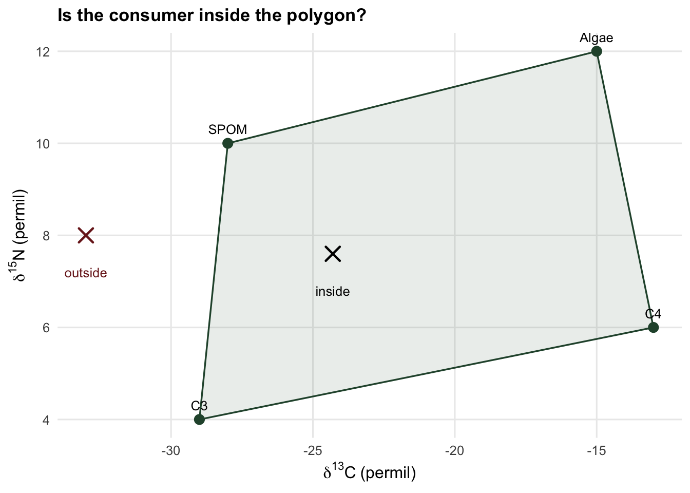
A non-negative mixture of the sources can only land inside their convex hull. If the discrimination-corrected consumer falls outside that polygon, no valid diet exists, and yet the sampler will still return a posterior, often a narrow and confident one. The check is geometric and takes a moment; skipping it is how impossible fits get reported as findings.
```{r}
#| label: feasibility
inpoly <- function(pt, poly) {
  n <- nrow(poly); inside <- FALSE; j <- n
  for (i in 1:n) {
    xi <- poly[i, 1]; yi <- poly[i, 2]; xj <- poly[j, 1]; yj <- poly[j, 2]
    if (((yi > pt[2]) != (yj > pt[2])) &&
        (pt[1] < (xj - xi) * (pt[2] - yi) / (yj - yi) + xi)) inside <- !inside
    j <- i
  }
  inside
}
poly <- Smu[chull(Smu), ]
consumer_in  <- c(d13C = -24.3, d15N = 7.6)              # a plausible consumer
consumer_out <- c(d13C = -33,   d15N = 8)                # more depleted than any source
c(inside = inpoly(consumer_in, poly), outside = inpoly(consumer_out, poly))
```
The second consumer sits at `d13C = -33`, more depleted than every source, so it is outside the polygon: no non-negative diet can reach it. Fit it anyway and read what comes back.
```{r}
#| label: outside-fit
set.seed(701)
y_out <- cbind(rnorm(20, consumer_out["d13C"], res[1]), rnorm(20, consumer_out["d15N"], res[2]))
fit_out <- mix_mh(y_out, Smu, Ssd, res, seed = 702)
do <- fit_out$draws; colnames(do) <- rownames(Smu)
spom_mean <- round(mean(do[, "SPOM"]), 3)
spom_sd <- round(sd(do[, "SPOM"]), 3)
round(rbind(mean = colMeans(do), sd = apply(do, 2, sd)), 3)
```
The fit is emphatic: it assigns `r spom_mean` of the diet to SPOM with a posterior standard deviation of only `r spom_sd`. Taken at face value that reads as a precise, near-certain result. It is an artefact. The sampler cannot reach the consumer with any real mixture, so it collapses onto the single source nearest the consumer in the isotope plane and reports false confidence. Without the polygon check, you would report "SPOM dominates the diet" from a consumer that no combination of these sources can produce. A concentrated posterior on an infeasible consumer is a warning, not a result.
```{r}
#| label: fig-feasibility
#| echo: false
#| fig-cap: "The mixing polygon with a feasible consumer (inside) and an infeasible one (outside, in red). The outside consumer is more depleted in carbon than any source, so no non-negative mixture reaches it. A mixing model fitted to it returns a confident but meaningless posterior."
#| fig-alt: "A d13C versus d15N biplot with four sources forming a polygon. One consumer sits inside; a red consumer sits to the left, clearly outside the polygon."
hull_df <- as.data.frame(rbind(poly, poly[1, ]))
sd_df <- data.frame(Smu, lab = rownames(Smu))
ggplot() +
geom_polygon(data = hull_df, aes(d13C, d15N), fill = te_green, alpha = 0.10,
colour = te_green, linewidth = 0.6) +
geom_point(data = sd_df, aes(d13C, d15N), colour = te_green, size = 3) +
geom_text(data = sd_df, aes(d13C, d15N, label = lab), vjust = -1, size = 3.4) +
geom_point(aes(consumer_in["d13C"], consumer_in["d15N"]), shape = 4, size = 4, stroke = 1.2) +
annotate("text", x = consumer_in["d13C"], y = consumer_in["d15N"] - 0.8,
label = "inside", size = 3.4) +
geom_point(aes(consumer_out["d13C"], consumer_out["d15N"]), shape = 4, size = 4,
stroke = 1.2, colour = "#7a1f1f") +
annotate("text", x = consumer_out["d13C"], y = consumer_out["d15N"] - 0.8,
label = "outside", size = 3.4, colour = "#7a1f1f") +
labs(x = expression(delta^13 * C~"(permil)"), y = expression(delta^15 * N~"(permil)"),
title = "Is the consumer inside the polygon?") +
theme_te()
```
## Check two: is the posterior driven by the data or the prior?
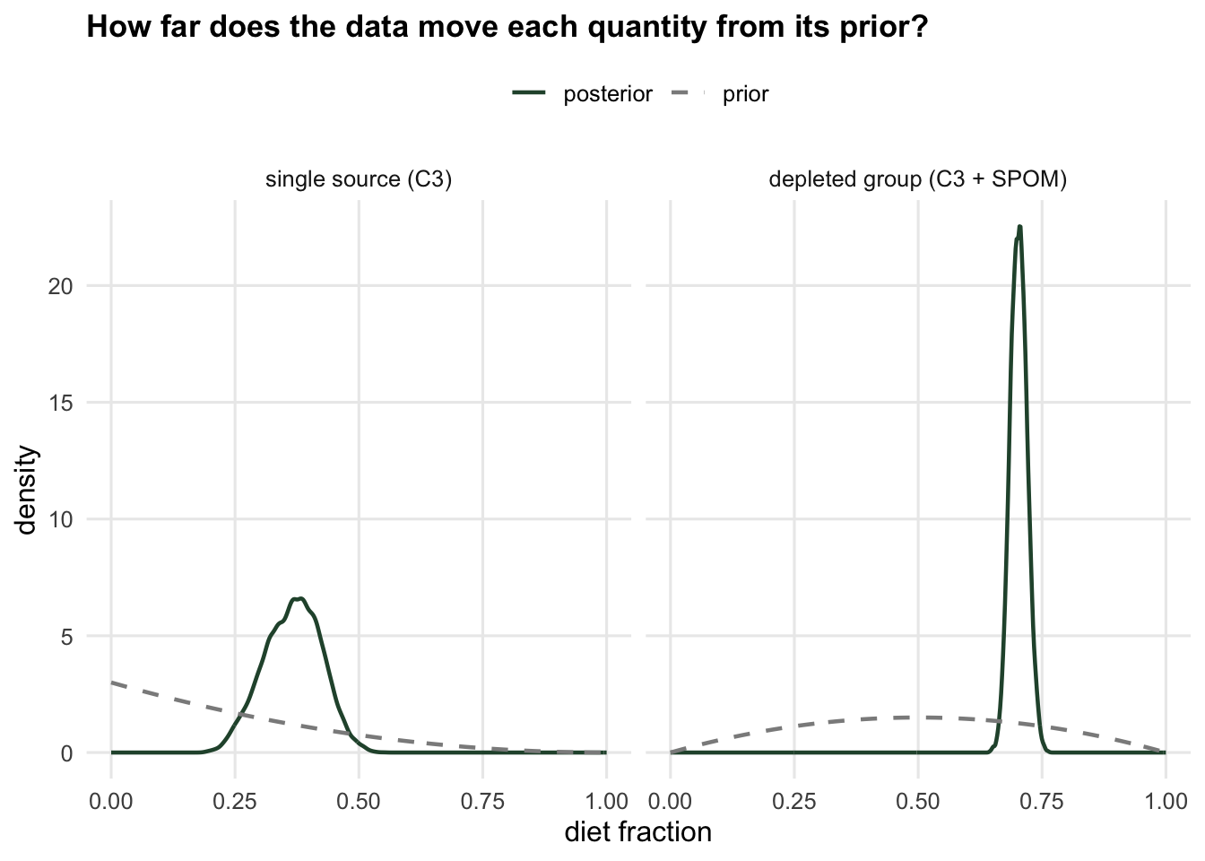
A broad posterior might mean the data are weakly informative, or it might mean you are mostly seeing the prior. The flat Dirichlet is not flat on the individual fractions: for four sources, each fraction has a Beta(1, 3) prior with a standard deviation near 0.19. A useful diagnostic is how much the data shrink that: compare the prior standard deviation to the posterior standard deviation. A quantity the data barely touch stays close to its prior width; a quantity the data pin down shrinks a lot.
```{r}
#| label: prior-sensitivity
p_true <- c(0.40, 0.10, 0.20, 0.30); mu_in <- as.numeric(t(Smu) %*% p_true)
set.seed(303)
y_in <- cbind(rnorm(20, mu_in[1], res[1]), rnorm(20, mu_in[2], res[2]))
fit_in <- mix_mh(y_in, Smu, Ssd, res, seed = 404)
d <- fit_in$draws; colnames(d) <- rownames(Smu)
J <- 4
prior_sd_ind <- sqrt((J - 1) / (J^2 * (J + 1)))          # Beta(1, J-1): single source
prior_sd_agg <- sqrt(2 * (J - 2) / (J^2 * (J + 1)))      # Beta(2, J-2): sum of two sources
g <- d[, "C3"] + d[, "SPOM"]                             # the depleted group
shrink_ind <- round(prior_sd_ind / mean(apply(d, 2, sd)), 1)
shrink_agg <- round(prior_sd_agg / sd(g), 1)
c(prior_sd_individual = round(prior_sd_ind, 3), posterior_sd_individual = round(mean(apply(d, 2, sd)), 3),
  shrink_individual = shrink_ind)
c(prior_sd_aggregate = round(prior_sd_agg, 3), posterior_sd_aggregate = round(sd(g), 3),
  shrink_aggregate = shrink_agg)
```
The individual fractions shrink by about `r shrink_ind` times relative to their prior; the depleted group shrinks by `r shrink_agg` times. The data inform the group far more sharply than the individual sources, but the individual posteriors are still much narrower than their prior, so by this check alone they would not look like assumptions. Their weakness is the one check three comes back to: the two tracer means alone cannot separate C3 from SPOM, and a narrow posterior does not show that they can. If a fraction's posterior barely shrinks from its prior, you are reporting an assumption, not a measurement.
```{r}
#| label: fig-prior
#| echo: false
#| fig-cap: "Prior (dashed) against posterior (solid) for a single source and for the depleted group. The individual source posterior is much narrower than its broad prior. The group posterior is narrower again, far tighter than its prior, and sits near the true value, so the data, not the prior, are speaking."
#| fig-alt: "Two panels. Left: a broad dashed prior curve and a much narrower solid posterior for one source. Right: a broad dashed prior and a very narrow solid posterior for the group, near the true value."
xx <- seq(0, 1, length.out = 400)
prior_ind <- dbeta(xx, 1, J - 1); prior_agg <- dbeta(xx, 2, J - 2)
pf <- rbind(
data.frame(x = xx, dens = prior_ind, kind = "prior", panel = "single source (C3)"),
data.frame(x = density(d[, "C3"], from = 0, to = 1)$x,
dens = density(d[, "C3"], from = 0, to = 1)$y, kind = "posterior", panel = "single source (C3)"),
data.frame(x = xx, dens = prior_agg, kind = "prior", panel = "depleted group (C3 + SPOM)"),
data.frame(x = density(g, from = 0, to = 1)$x,
dens = density(g, from = 0, to = 1)$y, kind = "posterior", panel = "depleted group (C3 + SPOM)"))
pf$panel <- factor(pf$panel, levels = c("single source (C3)", "depleted group (C3 + SPOM)"))
ggplot(pf, aes(x, dens, colour = kind, linetype = kind)) +
geom_line(linewidth = 0.8) +
facet_wrap(~panel) +
scale_colour_manual(values = c(prior = "grey55", posterior = te_green)) +
scale_linetype_manual(values = c(prior = "dashed", posterior = "solid")) +
labs(x = "diet fraction", y = "density", colour = NULL, linetype = NULL,
title = "How far does the data move each quantity from its prior?") +
theme_te() + theme(legend.position = "top")
```
## Check three: is the resolvable quantity stable across aggregation choices?
The [Bayesian post](../bayesian-isotope-mixing-models/) showed that summing the posterior draws for two sources that trade off against each other gives a well-determined group contribution. A quick stability check is to reach the same quantity by a different route: instead of summing draws afterwards (a posteriori), merge the two sources into one before fitting (a priori) and refit with three sources. If the group contribution is real and the merged source is a fair stand-in for the two it replaces, the two routes should agree.
```{r}
#| label: aggregate-check
Smu3 <- rbind(Depleted = colMeans(Smu[c("C3", "SPOM"), ]), C4 = Smu["C4", ], Algae = Smu["Algae", ])
Ssd3 <- rbind(Depleted = sqrt(colMeans(Ssd[c("C3", "SPOM"), ]^2)), C4 = Ssd["C4", ], Algae = Ssd["Algae", ])
fit3 <- mix_mh(y_in, Smu3, Ssd3, res, alpha = rep(1, 3), seed = 808)
d3 <- fit3$draws; colnames(d3) <- rownames(Smu3)
post_hoc <- round(c(mean = mean(g), sd = sd(g)), 3)
a_priori <- round(c(mean = mean(d3[, "Depleted"]), sd = sd(d3[, "Depleted"])), 3)
rbind(a_posteriori = post_hoc, a_priori = a_priori, truth = c(mean = 0.70, sd = NA))
```
Both routes put the depleted contribution at a posterior mean of about 0.70 with nearly the same spread, and both bracket the true value. Here the group contribution does not depend on whether you merge the sources before or after fitting. Part of that agreement is built in: the merged source sits halfway between C3 and SPOM, and the simulated diet splits the group between them fairly evenly. With a lopsided split the merged source would be a poor stand-in for the two it replaces, and the routes could disagree even about a group the data pin down, so agreement supports a group contribution only when the merged source is a fair stand-in. Contrast that with the individual C3 and SPOM fractions, which the two tracer means alone cannot separate and which shift when the assumed source spreads change: those are the quantities to leave out of the conclusions.
## Putting the checks together
Run all three before believing a mixing model. Is the consumer inside the mixing polygon, so a valid diet exists at all? Does the posterior for each reported quantity shrink meaningfully from its prior, so you are reading data rather than assumption? And is the quantity stable to how sources are grouped, so it is not an artefact of one arbitrary aggregation? A fit that passes all three is worth reporting, as long as what you report is a quantity the tracers can resolve; a fit that fails any of them is telling you to fix the study design, add tracers, or report a coarser quantity, not to trust the numbers as they stand.
## Honest limits
These are minimal, transparent versions of checks that mature tools formalise. The polygon test here uses source means; a fuller version simulates the mixing region accounting for source and discrimination uncertainty, which can shrink the feasible area. The prior-shrinkage diagnostic is a rule of thumb, not a formal model comparison. And agreement between the two aggregation routes confirms a quantity is stable, not that it is unbiased, since a wrong discrimination factor or a missing source would bias both routes together. The checks catch two of the common, fatal mistakes, an impossible consumer and a prior masquerading as a result, but not by themselves a third, an unresolvable fraction read as if it were pinned down: the individual C3 and SPOM fractions here pass the first two checks, and what marks them is that the two tracer means alone cannot separate C3 from SPOM. The checks do not substitute for a good sampling design and honest sources.
## References
Phillips DL, Gregg JW 2003 Oecologia 136:261-269 (10.1007/s00442-003-1218-3).
Phillips DL, Inger R, Bearhop S, Jackson AL, Moore JW, Parnell AC, Semmens BX, Ward EJ 2014 Canadian Journal of Zoology 92:823-835 (10.1139/cjz-2014-0127).
Stock BC, Jackson AL, Ward EJ, Parnell AC, Phillips DL, Semmens BX 2018 PeerJ 6:e5096 (10.7717/peerj.5096).
Moore JW, Semmens BX 2008 Ecology Letters 11:470-480 (10.1111/j.1461-0248.2008.01163.x).
## Related tutorials
- [Stable isotope mixing models in R](../isotope-mixing-models-in-r/)
- [Bayesian stable isotope mixing models](../bayesian-isotope-mixing-models/)
- [Discrimination and concentration in mixing models](../discrimination-and-concentration-in-mixing/)
- [Checking an isotopic niche analysis](../checking-an-isotopic-niche-analysis/)