Stable isotope mixing models in R

The geometry behind stable isotope mixing models in R: mass balance, the mixing polygon, and why more diet sources than tracers leave the answer undetermined.

A stable isotope mixing model answers a simple-sounding question: a consumer’s tissue carries a carbon and nitrogen isotope signature, several potential food sources each carry their own, so what fraction of the diet came from each source? The machinery that answers this looks like statistics, but underneath it is geometry, and the geometry sets a hard limit that no amount of clever fitting removes. This post builds the mixing model from mass balance, solves the case where the geometry gives one answer, and shows the case where it gives infinitely many.

Everything here is base R plus ggplot2. Later posts in this cluster add a Bayesian version, the assumed inputs that quietly drive the result, and the checks worth running before you trust a mixing model.

Sources, a consumer, and the mixing space

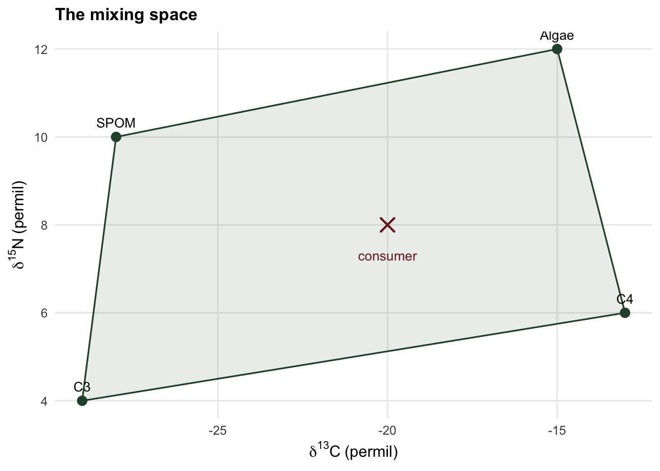
Two tracers are the classic pair: d13C on one axis, d15N on the other. Each source is a point in this plane, and a consumer that eats a mixture of the sources sits at a weighted average of their positions. The set of points a consumer could occupy, given non-negative diet fractions that sum to one, is the convex hull of the source points: the mixing polygon. A consumer inside the polygon has at least one feasible diet; a consumer outside it has none.

# Four sources, already corrected to the consumer's trophic level.
# Columns are the two tracers (d13C, d15N).
src <- rbind(C3    = c(-29,  4),
             C4    = c(-13,  6),
             Algae = c(-15, 12),
             SPOM  = c(-28, 10))
colnames(src) <- c("d13C", "d15N")
consumer <- c(d13C = -20, d15N = 8)
src

      d13C d15N
C3     -29    4
C4     -13    6
Algae  -15   12
SPOM   -28   10

Figure 1: Four sources (points) with their mixing polygon (the convex hull), and one consumer (cross) sitting inside it. Any consumer inside the polygon can be written as a non-negative mixture of the sources; a consumer outside it cannot.

When the geometry gives one answer

Write the diet fractions as a vector p, one entry per source. Mass balance says that for each tracer, the consumer value equals the fraction-weighted average of the source values, and the fractions sum to one. With J sources and T tracers, that is T + 1 linear equations in J unknowns:

\[ \sum_j p_j\, s_{jt} = y_t \quad (t = 1 \ldots T), \qquad \sum_j p_j = 1 . \]

With two tracers and three sources, that is three equations in three unknowns: a square system with a unique solution. The solution is just the consumer’s position expressed in the coordinate system of the three source points (its barycentric coordinates). Solving is a one-liner.

S3 <- src[c("C3", "C4", "Algae"), ]        # drop the fourth source
M3 <- rbind(t(S3), 1)                       # 3 x 3: two tracer rows, one sum-to-one row
y3 <- c(consumer, 1)
p3 <- solve(M3, y3)
p3_c3    <- round(p3[1], 3)
p3_c4    <- round(p3[2], 3)
p3_algae <- round(p3[3], 3)
round(p3, 3)

   C3    C4 Algae 
 0.38  0.16  0.46 

The three sources give a single diet: 0.38 C3, 0.16 C4, 0.46 Algae. All three fractions land in [0, 1], so the answer is feasible, and the reconstruction is exact (multiply the sources by these fractions and you recover the consumer). With as many sources as the geometry can carry, the mixing model behaves like ordinary linear algebra: one input, one output.

When the geometry gives infinitely many answers

Add a fourth source and nothing about the data changes, but the system does. Now there are three equations and four unknowns. The matrix has rank three, so there is one degree of freedom: the solutions form a line, and where that line crosses the region of non-negative fractions is a whole segment, not a point.

M4 <- rbind(t(src), 1)                       # 3 x 4
dof <- ncol(M4) - qr(M4)$rank
pp <- qr.solve(M4, c(consumer, 1))           # one particular solution
ns <- svd(M4, nu = 0, nv = 4)$v[, 4]         # direction along the solution line
# walk along the line: p(t) = pp + t * ns, keep only t with all fractions >= 0
t_lo <- -Inf; t_hi <- Inf
for (j in 1:4) {
  if (ns[j] >  1e-12) t_lo <- max(t_lo, (-pp[j]) / ns[j])
  if (ns[j] < -1e-12) t_hi <- min(t_hi, (-pp[j]) / ns[j])
}
feas <- rbind(end_A = pp + t_lo * ns, end_B = pp + t_hi * ns)
colnames(feas) <- rownames(src)
dof

[1] 1

round(feas, 3)

        C3    C4 Algae  SPOM
end_A 0.38 0.160 0.460 0.000
end_B 0.00 0.512 0.024 0.463

rng <- apply(feas, 2, range)
width <- rng[2, ] - rng[1, ]
spom_lo <- round(rng[1, "SPOM"], 2); spom_hi <- round(rng[2, "SPOM"], 2)
wid_spom <- round(width["SPOM"], 2)
wid_algae <- round(width["Algae"], 2)
round(rbind(low = rng[1, ], high = rng[2, ], width = width), 3)

        C3    C4 Algae  SPOM
low   0.00 0.160 0.024 0.000
high  0.38 0.512 0.460 0.463
width 0.38 0.352 0.436 0.463

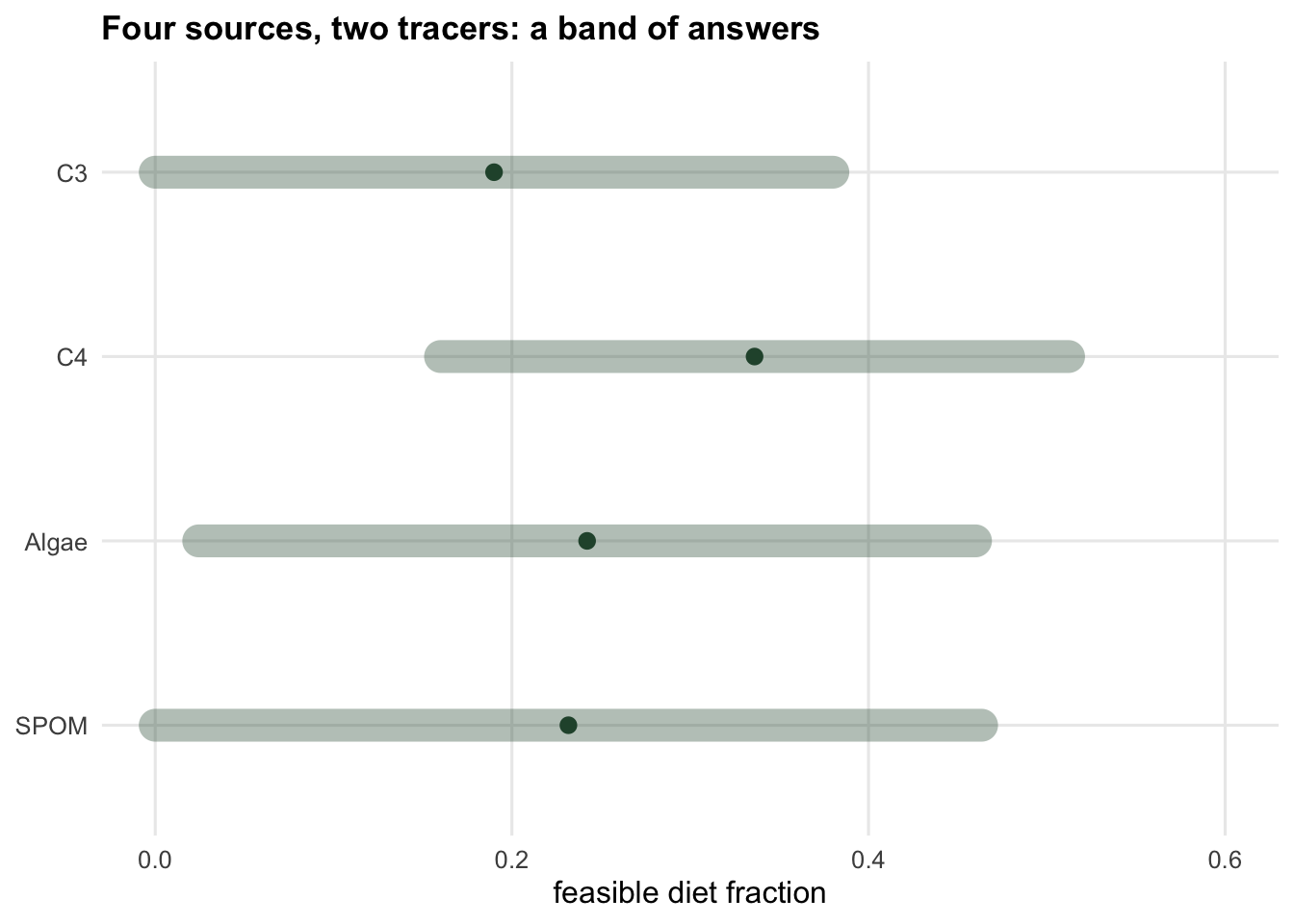
Both rows of feas fit the consumer exactly; they are two ends of a segment of equally valid diets. Read the columns and the problem is stark. The SPOM fraction can be anywhere from 0 to 0.46 (a range of 0.46) while still reproducing the consumer’s isotopes to the last decimal. Algae ranges over 0.44. Two tracers simply do not carry enough information to pin four sources: the consumer’s single point in the plane is consistent with a continuum of mixtures.

Figure 2: The feasible diets for the four-source problem, as fractions per source. Each source’s bar spans the full range of values consistent with the consumer’s isotopes; every point along a bar reproduces the data exactly. Two tracers leave a wide band of equally good answers.

The single-point estimate in the middle of each bar is not wrong so much as arbitrary: it is one interior solution chosen by the numerical routine, and a different routine would return a different one. Reporting it as “the answer” hides the range. Later this cluster shows how a Bayesian model reports the whole band honestly, and why grouping sources with similar signatures is often the only way to get a resolvable quantity.

A consumer outside the polygon

Mass balance with non-negative fractions can only produce consumers inside the mixing polygon. If the corrected consumer falls outside it, no feasible diet exists, and the linear routine will happily return a solution with negative fractions. The check is geometric: is the consumer inside the convex hull of the sources?

inpoly <- function(pt, poly) {           # ray-casting point-in-polygon
  n <- nrow(poly); inside <- FALSE; j <- n
  for (i in 1:n) {
    xi <- poly[i, 1]; yi <- poly[i, 2]; xj <- poly[j, 1]; yj <- poly[j, 2]
    if (((yi > pt[2]) != (yj > pt[2])) &&
        (pt[1] < (xj - xi) * (pt[2] - yi) / (yj - yi) + xi)) inside <- !inside
    j <- i
  }
  inside
}
poly <- src[chull(src), ]
out_consumer <- c(d13C = -31, d15N = 8)     # more depleted than any source
c(inside = inpoly(consumer, poly), outside = inpoly(out_consumer, poly))

 inside outside 
   TRUE   FALSE 

A consumer at d13C = -31 sits to the left of every source and lands outside the polygon. Because all four sources have d13C values of -29 or higher, no weighted average of them can reach -31: the fractions that would try are negative. A negative diet fraction is the signature of an impossible mixing problem, and it usually means a missing source, a wrong discrimination correction, or source values measured on the wrong scale. The mixing model cannot rescue a consumer that its sources cannot bracket.

Where to go next

The geometry is the frame; everything else in this cluster hangs on it. The Bayesian version turns the feasible band into a posterior distribution and adds source uncertainty. The assumed inputs post shows that the correction you apply to the sources before any of this, the trophic discrimination factor, moves the result more than the data do. And the checking post collects the diagnostics: is the consumer inside the polygon, is the posterior informed by data, and which contributions are actually resolvable.

Honest limits

The single-answer case is the exception, not the rule. Real studies usually have more candidate sources than tracers, so the underdetermined case is the normal one, and its wide band of solutions is a feature of the geometry, not a failure of the method. Adding tracers (a third isotope, fatty acids) is the direct fix, because each independent tracer adds a dimension to the mixing space; grouping sources with overlapping signatures is the other. What you cannot do is squeeze a unique diet out of two tracers and four distinct sources, however sophisticated the fitting routine.

Related tutorials

• Bayesian stable isotope mixing models
• Discrimination and concentration in mixing models
• Checking a stable isotope mixing model
• Log-ratio transformations for compositional data

References

Phillips DL, Gregg JW 2001 Oecologia 127:171-179.

Phillips DL, Gregg JW 2003 Oecologia 136:261-269 (10.1007/s00442-003-1218-3).

Phillips DL, Inger R, Bearhop S, Jackson AL, Moore JW, Parnell AC, Semmens BX, Ward EJ 2014 Canadian Journal of Zoology 92:823-835 (10.1139/cjz-2014-0127).

Post DM 2002 Ecology 83:703-718.

## References

Phillips DL, Gregg JW 2001 Oecologia 127(2):171-179 (10.1007/s004420000578).