Discrimination and concentration in mixing models

In stable isotope mixing models the assumed discrimination factor and elemental concentrations can drive the diet estimate more than the consumer data do.

Corrected 14 October 2026: the post said the nitrogen-rich invertebrate dominates the nitrogen isotope signal, although it supplies the smallest share of the consumer’s nitrogen, and now says that this share is well above its share of the diet; a sentence still called the discrimination factor, not the data, the thing to worry about in general and now limits this to the example; and the post said the checking post turns the sensitivity checks into a routine, whereas none of its checks varies the discrimination factor or the concentrations, and it now says so.

Corrected 7 October 2026: a sentence and a plot title still said that ignoring concentration overestimates the rich source, and now limit this to the example; the comparison with the Bayesian post now uses its fit to these same three sources, not its four-source fit, whose width comes from the geometry; and the claim that the discrimination factor outweighs consumer sampling in most studies is now made for this example only.

Corrected 30 September 2026: the post said that ignoring concentration always overcounts high-concentration sources and undercounts low-concentration ones; the direction of that bias depends on where the sources sit in isotope space, and the post now says so.

A stable isotope mixing model takes source values, a consumer value, and returns diet fractions. Two of those inputs are usually treated as fixed and known, when in fact they are assumed: the trophic discrimination factor that shifts a consumer’s isotopes away from its diet, and the elemental concentration of each source. This post shows, with the same tidy examples as the rest of the mixing-model cluster, that these assumptions move the answer more than the consumer measurements do. If you report a mixing model without stating them, you may have hidden the biggest source of uncertainty in the result.

The discrimination factor is an assumption, not a measurement

A consumer is not isotopically identical to its food. As nitrogen passes up a trophic level, the heavier isotope is retained, so a consumer’s d15N is typically a few permil above its diet; carbon shifts much less. That offset is the trophic discrimination factor (TDF), and every mixing model corrects the sources by it before solving. The catch is that the TDF is not measured on your animal; it is borrowed from feeding experiments on other species, and it varies. The classic nitrogen value is about 3.4 permil, but published estimates scatter with a standard deviation near one permil. Treating a borrowed, uncertain number as exact is where mixing models quietly go wrong.

Take a determined three-source problem so the geometry is not the issue: with the correct TDF, the model returns the true diet exactly. Generate a consumer from a known diet and the true discrimination factor.

S3 <- rbind(C3 = c(-29, 4), C4 = c(-13, 6), Algae = c(-15, 12))
colnames(S3) <- c("d13C", "d15N")
p_true <- c(0.40, 0.30, 0.30)
TDF_true <- c(0.5, 3.4)                                  # true discrimination (d13C, d15N)
consumer <- as.numeric(t(S3) %*% p_true) + TDF_true      # consumer = diet mean + TDF
# solve for diet given an ASSUMED discrimination factor
solve_p <- function(TDF) {
  Sc <- sweep(S3, 2, TDF, "+")                           # correct sources by assumed TDF
  as.numeric(solve(rbind(t(Sc), 1), c(consumer, 1)))
}
round(solve_p(TDF_true), 3)                              # correct TDF -> true diet

[1] 0.4 0.3 0.3

With the true TDF the model returns exactly 40% C3, 30% C4, 30% Algae. Now do the honest thing and admit you do not know the nitrogen discrimination to better than about a permil. Sweep the assumed value across a realistic range and watch the estimate move.

grid <- c(2.4, 2.9, 3.4, 3.9, 4.4)                       # assumed TDF_N, true value is 3.4
est <- t(sapply(grid, function(tn) solve_p(c(0.5, tn))))
colnames(est) <- rownames(S3); rownames(est) <- paste0("TDF_N=", grid)
algae_lo <- round(est["TDF_N=2.4", "Algae"], 3)
algae_hi <- round(est["TDF_N=4.4", "Algae"], 3)
algae_shift <- round(algae_lo - algae_hi, 3)
c4_shift <- round(est["TDF_N=4.4", "C4"] - est["TDF_N=2.4", "C4"], 3)
round(est, 3)

            C3   C4 Algae
TDF_N=2.4 0.38 0.16  0.46
TDF_N=2.9 0.39 0.23  0.38
TDF_N=3.4 0.40 0.30  0.30
TDF_N=3.9 0.41 0.37  0.22
TDF_N=4.4 0.42 0.44  0.14

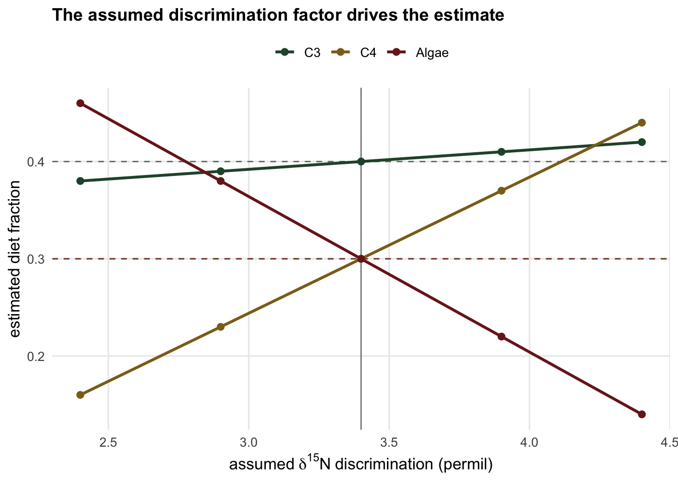
The true diet appears only in the middle row, at the exactly-correct TDF. One permil either side and the Algae estimate runs from 0.46 down to 0.14, a shift of 0.32; C4 moves by 0.28 in the opposite direction. That is about a third of the whole range a diet fraction can take, produced not by any change in the data but by a plus-or-minus-one-permil guess about a physiological constant. C3 barely moves, because its distance from the other two sources is on the carbon axis, which the nitrogen sweep does not touch.

Figure 1: Estimated diet fractions as the assumed nitrogen discrimination factor is swept across a realistic one-permil band around the true value (vertical line). The C4 and Algae estimates each swing by roughly three tenths of the zero-to-one range; only at the correct value is the true diet (dashed) recovered. The data never changed.

Compare this swing to the posterior width from consumer noise in the Bayesian post: there, noisy consumer measurements on these same three sources, with this same diet, gave posterior standard deviations of only a hundredth or two. Here, a routine one-permil uncertainty in the discrimination factor moves the point estimate by a few tenths, an order of magnitude larger. In this example the discrimination factor, not the data, is the thing to worry about, and the way to handle it is to propagate its uncertainty (put a prior on it) rather than plug in a single borrowed number.

Concentration dependence: not all sources mix equally

The standard mixing model assumes each source contributes the same fraction to every tracer. That is only true if the sources have similar elemental concentrations. When one source is much richer in an element, it contributes disproportionately to that tracer: a nitrogen-rich prey item pulls the consumer’s d15N toward itself out of proportion to its dietary mass. Ignoring this, the model reads the pulled signal as a change in the diet; in the example below it shows up as more of the rich source, but which way the estimate moves depends on where the sources sit in isotope space.

Set up three sources whose nitrogen content differs, a plant low in nitrogen up to an invertebrate more than twice as rich, and mix them by a known biomass diet using concentration-weighted mass balance.

Sc <- rbind(Plant = c(-30, 2), Detritus = c(-20, 5), Invert = c(-24, 10))
colnames(Sc) <- c("d13C", "d15N")
conc <- rbind(Plant = c(C = 44, N = 2.5), Detritus = c(C = 42, N = 4), Invert = c(C = 45, N = 6.5))
p_bio <- c(0.55, 0.30, 0.15)                             # true diet by biomass
# concentration-weighted mixing: each element weighted by mass x concentration
w_c <- p_bio * conc[, "C"]; w_n <- p_bio * conc[, "N"]
consumer_c <- c(d13C = sum(w_c * Sc[, "d13C"]) / sum(w_c),
                d15N = sum(w_n * Sc[, "d15N"]) / sum(w_n))
round(consumer_c, 2)

  d13C   d15N 
-26.18   5.21 

Now estimate the diet two ways: the naive model that ignores concentration (ordinary mass balance), and the concentration-weighted model that accounts for it.

# naive: plain linear mixing, concentrations assumed equal
p_naive <- as.numeric(solve(rbind(t(Sc), 1), c(consumer_c, 1)))
names(p_naive) <- rownames(Sc)
# concentration-weighted: recover the biomass diet by minimising the weighted mismatch
obj <- function(q) {
  p <- c(q, 1 - sum(q)); if (any(p < 0)) return(1e6)
  wc <- p * conc[, "C"]; wn <- p * conc[, "N"]
  (sum(wc * Sc[, "d13C"]) / sum(wc) - consumer_c["d13C"])^2 +
  (sum(wn * Sc[, "d15N"]) / sum(wn) - consumer_c["d15N"])^2
}
op <- optim(c(0.33, 0.33), obj, control = list(reltol = 1e-12))
p_weighted <- c(op$par, 1 - sum(op$par))
inv_naive <- round(p_naive["Invert"], 3)
inv_bias <- round(100 * (p_naive["Invert"] - p_bio[3]) / p_bio[3])
rbind(truth = p_bio, naive = round(p_naive, 3), weighted = round(p_weighted, 3))

         Plant Detritus Invert
truth    0.550    0.300  0.150
naive    0.484    0.183  0.333
weighted 0.550    0.300  0.150

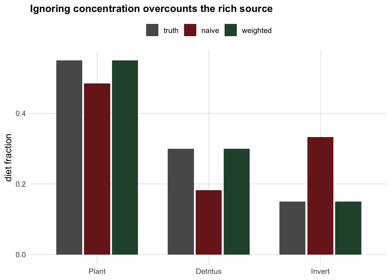
The concentration-weighted model recovers the true biomass diet (55% Plant, 30% Detritus, 15% Invert). The naive model does not: it puts the invertebrate at 0.333 instead of 0.15, an overestimate of 122 per cent. The invertebrate is the most nitrogen-rich source, so its share of the consumer’s nitrogen, which sets its weight in the d15N mass balance, is well above its share of the diet, and a model that assumes equal concentrations attributes that pulled signal to a larger invertebrate contribution. The bias is systematic, but its direction is not fixed: here the nitrogen-rich invertebrate is overcounted, while with the sources placed differently in isotope space the same concentrations can push a rich source down instead.

Figure 2: True biomass diet against the naive (concentration-ignoring) and concentration-weighted estimates. The naive model overstates the nitrogen-rich invertebrate and understates the rest; weighting by elemental concentration recovers the truth. The isotope data are identical in both fits.

Where to go next

Both of these are inputs you supply, not things the model estimates, and both can dominate the result. The practical response is the same for each: do not plug in a single number and treat the output as precise. Put a prior on the discrimination factor and let it propagate, use measured elemental concentrations rather than assuming they are equal, and check how sensitive your conclusion is to both. The checking post adds a short routine of other checks you can run on any fit, although none of them varies the discrimination factor or the concentrations. The Bayesian post shows how a Bayesian fit carries source uncertainty through to the diet estimate.

Honest limits

The discrimination sweep here used a fixed carbon TDF and moved only nitrogen, and the concentration example used two tracers and three sources so the geometry stayed clean. Real studies have both problems at once: uncertain discrimination on every tracer, unequal concentrations, and more sources than tracers. The point is not the exact numbers, which depend on the isotopic spacing of your particular sources, but the comparison: in this example the discrimination factor is a larger source of error than the consumer sampling, and unmodelled concentration differences bias the answer systematically, in a direction set by where the sources sit. Neither is fixed by collecting more consumer samples.

References

Caut S, Angulo E, Courchamp F 2009 Journal of Applied Ecology 46(2):443-453 (10.1111/j.1365-2664.2009.01620.x).

Phillips DL, Koch PL 2002 Oecologia 130(1):114-125 (10.1007/s004420100786).

Phillips DL, Inger R, Bearhop S, Jackson AL, Moore JW, Parnell AC, Semmens BX, Ward EJ 2014 Canadian Journal of Zoology 92(10):823-835 (10.1139/cjz-2014-0127).

Post DM 2002 Ecology 83(3):703-718 (10.1890/0012-9658(2002)083[0703:USITET]2.0.CO;2).

Related tutorials

• Stable isotope mixing models in R
• Bayesian stable isotope mixing models
• Checking a stable isotope mixing model
• Sensitivity and elasticity in matrix models

Reproducibility

• Code last run: 2026-10-15
• R version 4.5.3 (2026-03-11), aarch64-apple-darwin20
• Packages: ggplot2 4.0.3