Bayesian stable isotope mixing models

Build a Bayesian stable isotope mixing model from scratch in R with a Metropolis sampler, and read the wide, correlated posterior that two tracers produce.

Corrected 7 October 2026: the simulated consumers were drawn with the residual spread alone, less than the model assumes, so with many consumers the four-source posterior would settle on the wrong diet; they are now drawn with the spread the model assumes and every result has been rerun, which leaves the four-source chain slower to mix and its intervals a little wider. The more-data comparison is now averaged over several simulated data sets instead of resting on one pair, and the correlation plot no longer says the two depleted sources trade off one-for-one.

Corrected 1 October 2026: the post said the two depleted sources carry the largest loadings on the one free direction of the diet and so trade off most sharply; all four sources load on it with similar weight, SPOM and Algae the most, and the post now says which pair is most tightly locked depends on the spread the data leave in the other directions.

Corrected 30 September 2026: the post said part of the posterior width is fixed by the geometry and no consumer sample size removes it; in this model the width keeps shrinking with more consumers, because the known source spreads make the variance depend on the diet, and the post now says so and that this rests on the variance assumption.

The geometry post showed the problem: with two tracers and four sources, a consumer’s isotope signature is consistent with a whole band of diets, not one. A point estimate picks an arbitrary member of that band and hides the rest. A Bayesian mixing model does the honest thing instead: it reports the full band as a posterior distribution, so the uncertainty is visible rather than swept into a single number. This is what SIAR, MixSIR, and MixSIAR do. Here we build a small version from scratch, in base R, to see exactly where the width and the correlations come from.

The model

Each source has a mean isotope value and a spread; real sources are not points, they are clouds of measured individuals. The model treats the consumer’s tracer values as normal around the mixture mean, with a variance that combines the (fraction-weighted) source variances and a residual term:

\[ y_t \sim \mathcal{N}\!\left(\textstyle\sum_j p_j s_{jt},\ \ \textstyle\sum_j p_j^2 \sigma_{jt}^2 + \omega_t^2\right). \]

The diet fractions p live on the simplex (non-negative, sum to one), so the natural prior is a Dirichlet. A flat Dirichlet(1, …, 1) is the usual “uninformative” choice, uniform over the simplex. That is the whole model: a normal likelihood for the tracers and a Dirichlet prior for the fractions. Fitting it means sampling the posterior.

library(ggplot2)
theme_te <- function() {
  theme_minimal(base_size = 12) +
    theme(plot.title = element_text(face = "bold", size = 13),
          plot.background = element_rect(fill = "#f5f4ee", colour = NA),
          panel.background = element_rect(fill = "#f5f4ee", colour = NA),
          panel.grid.minor = element_blank())
}
te_green <- "#275139"
te_pal <- c("#275139", "#8c6d1f", "#7a1f1f", "#1f5c7a")
# Dirichlet density (log) and sampler; a small effective-sample-size helper.
ldir <- function(x, a) lgamma(sum(a)) - sum(lgamma(a)) + sum((a - 1) * log(pmax(x, 1e-12)))
rdir <- function(a) { g <- pmax(rgamma(length(a), a, 1), 1e-300); g / sum(g) }
ess <- function(x) {
  x <- x - mean(x); n <- length(x)
  r <- acf(x, lag.max = min(2000, n - 1), plot = FALSE)$acf[-1]
  k <- which(r < 0.05)[1]; if (is.na(k)) k <- length(r)
  rho <- r[1:max(1, k - 1)]; n / (1 + 2 * sum(rho))
}

A sampler in one function

Because the fractions are constrained to the simplex, an ordinary random walk would keep proposing invalid points. A cleaner move is a Dirichlet proposal centred on the current point: draw p* from a Dirichlet whose mean is the current p, with a concentration kappa that tunes the step size. The proposal is not symmetric, so the Metropolis-Hastings ratio needs the proposal densities in both directions; the flat prior cancels in the ratio. The whole sampler is short.

mix_mh <- function(y, Smu, Ssd, res, alpha = rep(1, nrow(Smu)),
                   kappa = 600, iter = 60000, burn = 12000, seed = 1) {
  n <- nrow(y); J <- nrow(Smu)
  loglik <- function(p) {
    mu <- as.numeric(t(Smu) %*% p)                       # mixture mean per tracer
    v  <- as.numeric(t(Ssd^2) %*% (p^2)) + res^2         # source + residual variance
    sum(dnorm(y, rep(mu, each = n), rep(sqrt(v), each = n), log = TRUE))
  }
  set.seed(seed)
  p <- rep(1 / J, J); ll <- loglik(p) + ldir(p, alpha)
  keep <- matrix(NA_real_, iter, J); acc <- 0
  for (t in 1:iter) {
    ap  <- pmax(kappa * p, 1e-3); ps <- rdir(ap)         # propose from Dirichlet(kappa * p)
    aps <- pmax(kappa * ps, 1e-3)
    lls <- loglik(ps) + ldir(ps, alpha)
    # Hastings ratio: likelihood + prior + reverse/forward proposal densities
    if (log(runif(1)) < (lls - ll) + ldir(p, aps) - ldir(ps, ap)) {
      p <- ps; ll <- lls; acc <- acc + 1
    }
    keep[t, ] <- p
  }
  list(draws = keep[(burn + 1):iter, , drop = FALSE], acc = acc / iter)
}

The 1e-3 floor on the Dirichlet parameters and the 1e-12 floor inside ldir matter: when a fraction is pushed to the edge of the simplex, log(0) would otherwise produce NaN and stall the chain. Guarding the logarithms keeps the sampler stable near the boundary.

Smu <- rbind(C3 = c(-29, 4), C4 = c(-13, 6), Algae = c(-15, 12), SPOM = c(-28, 10))
Ssd <- rbind(C3 = c(1.0, 0.8), C4 = c(1.2, 1.0), Algae = c(0.9, 1.1), SPOM = c(1.1, 0.9))
colnames(Smu) <- colnames(Ssd) <- c("d13C", "d15N")
res <- c(0.5, 0.4)                                       # residual SD per tracer

Does the sampler work? A determined test first

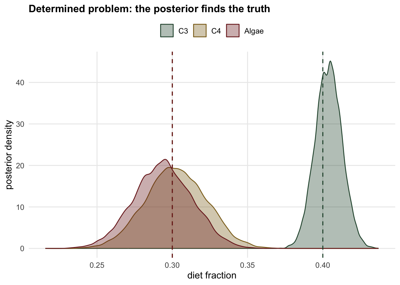
Before trusting any sampler on a hard problem, run it on an easy one where the answer is known. Three sources and two tracers is determined (the geometry post solved it exactly), so a consumer generated from a known diet should give a posterior that concentrates near that diet. Generate data from a diet of 40% C3, 30% C4, 30% Algae, drawing each consumer with the spread the model assumes (the fraction-weighted source spreads plus the residual), and fit.

S3 <- Smu[c("C3", "C4", "Algae"), ]; Sd3 <- Ssd[c("C3", "C4", "Algae"), ]
p_true3 <- c(0.40, 0.30, 0.30)
mu3 <- as.numeric(t(S3) %*% p_true3)
sd3 <- sqrt(as.numeric(t(Sd3^2) %*% p_true3^2) + res^2)   # spread the model assumes
set.seed(101)
y3 <- cbind(rnorm(30, mu3[1], sd3[1]), rnorm(30, mu3[2], sd3[2]))
fit3 <- mix_mh(y3, S3, Sd3, res, alpha = rep(1, 3), iter = 40000, burn = 8000, seed = 202)
cal_acc <- round(fit3$acc, 3)
cal_ess <- round(min(apply(fit3$draws, 2, ess)))
cal_means <- round(colMeans(fit3$draws), 3)
c(acceptance = cal_acc, min_ESS = cal_ess)

acceptance    min_ESS 
     0.396   1807.000 

rbind(posterior_mean = cal_means, truth = p_true3)

                [,1]  [,2]  [,3]
posterior_mean 0.406 0.306 0.288
truth          0.400 0.300 0.300

The acceptance rate is 0.396 and the smallest effective sample size across the three fractions is 1807, so the chain mixes well. The posterior means (0.406 C3, 0.306 C4, 0.288 Algae) sit close to the true diet. The sampler recovers a known answer when the geometry allows it. Now push it into the case that does not.

Figure 1: Posterior distributions for the determined three-source problem. Each fraction concentrates tightly around its true value (dashed line). When the geometry pins the answer, the Bayesian model finds it.

The underdetermined posterior

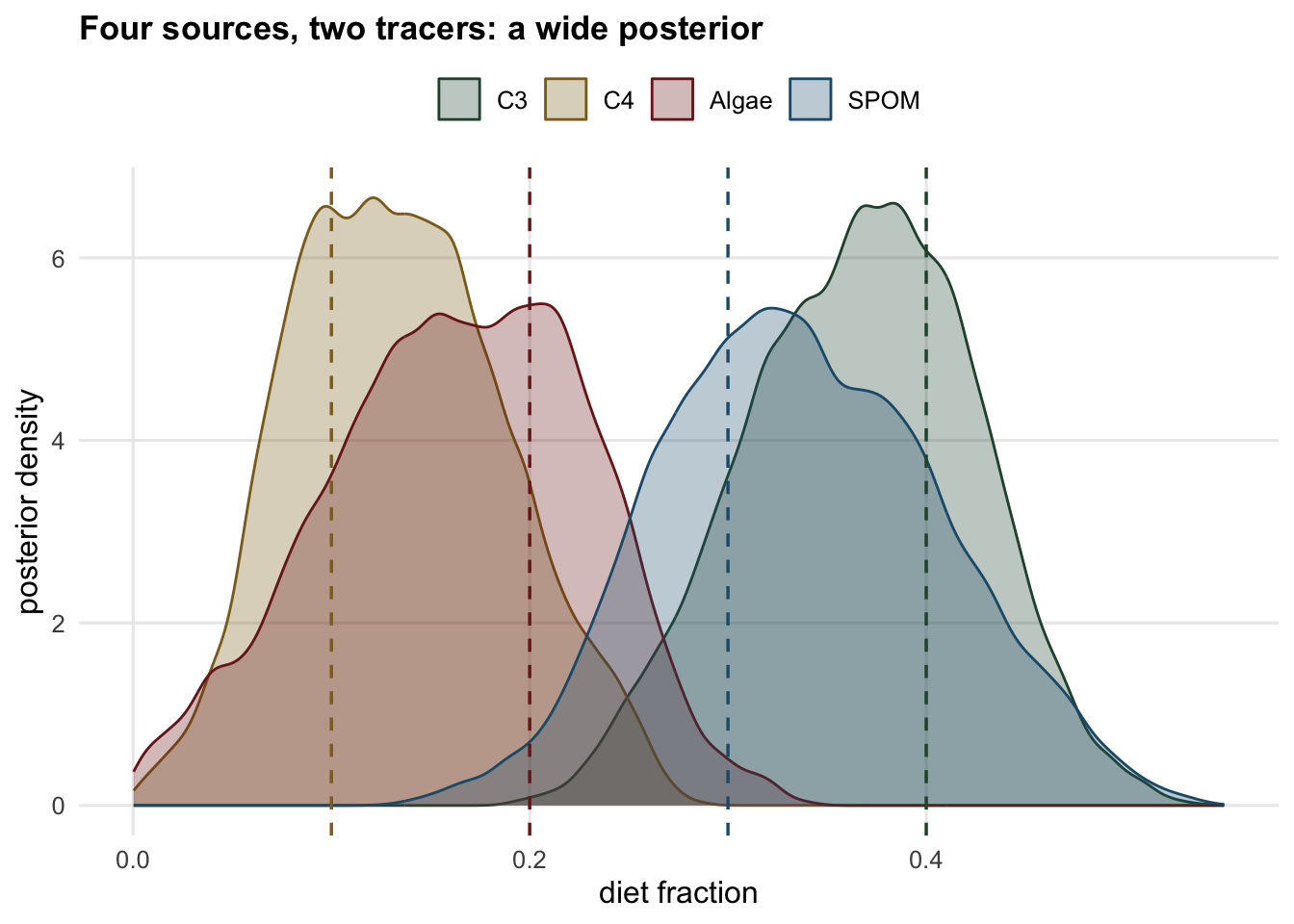
Bring back the fourth source. The consumer is generated in the same way from a diet of 40% C3, 10% C4, 20% Algae, 30% SPOM, but now four unknowns face three constraints. The sampler still runs; the posterior tells the real story.

p_true4 <- c(0.40, 0.10, 0.20, 0.30)
mu4 <- as.numeric(t(Smu) %*% p_true4)
sd4 <- sqrt(as.numeric(t(Ssd^2) %*% p_true4^2) + res^2)
set.seed(303)
y4 <- cbind(rnorm(20, mu4[1], sd4[1]), rnorm(20, mu4[2], sd4[2]))
fit4 <- mix_mh(y4, Smu, Ssd, res, iter = 60000, burn = 12000, seed = 404)
d <- fit4$draws
colnames(d) <- rownames(Smu)
u_acc <- round(fit4$acc, 3)
u_ess <- round(min(apply(d, 2, ess)))
post <- t(apply(d, 2, function(z) c(mean = mean(z), sd = sd(z),
                                    lo = quantile(z, 0.025), hi = quantile(z, 0.975))))
rownames(post) <- rownames(Smu)
sd_spom <- round(post["SPOM", "sd"], 3)
sd_c3 <- round(post["C3", "sd"], 3)
round(cbind(post, truth = p_true4), 3)

       mean    sd lo.2.5% hi.97.5% truth
C3    0.358 0.067   0.229    0.485   0.4
C4    0.141 0.061   0.024    0.256   0.1
Algae 0.156 0.075   0.013    0.299   0.2
SPOM  0.345 0.081   0.190    0.499   0.3

The chain mixes slowly along this broad posterior (acceptance 0.469, but a minimum effective sample size of only 91), so its summaries are rough. The SPOM fraction has a posterior standard deviation of 0.081 and a 95% credible interval roughly a third of the whole simplex wide; C3 is similar. Every one of these fractions has a true value comfortably inside its interval, so the model is not wrong, it is honestly uncertain. This width is the band from the geometry post, now expressed as probability.

Figure 2: Posterior distributions for the four-source problem. Each fraction is broad and its interval covers the true value (dashed line), but no fraction is pinned down. The width is the geometric ambiguity of two tracers and four sources, made explicit.

A single point estimate would hide all of this. The minimum-norm linear solution, for instance, returns one plausible-looking diet:

M <- rbind(t(Smu), 1)
b <- c(colMeans(y4), 1)
p_point <- as.numeric(t(M) %*% solve(M %*% t(M), b))     # minimum-norm solution
names(p_point) <- rownames(Smu)
round(p_point, 3)

   C3    C4 Algae  SPOM 
0.362 0.137 0.159 0.342 

Those four numbers look like an answer, but they are one arbitrary point inside the posterior cloud. Reporting them alone would imply a precision the data do not support.

Why the fractions trade off

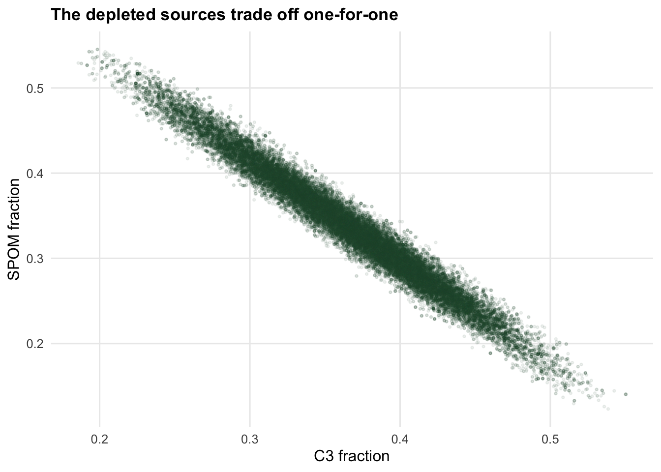
The fractions are not just individually uncertain, they are locked together. Look at the posterior correlations.

C <- cor(d); dimnames(C) <- list(rownames(Smu), rownames(Smu))
cor_sc <- round(C["SPOM", "C3"], 2)
round(C, 2)

         C3    C4 Algae  SPOM
C3     1.00 -0.93  0.94 -0.99
C4    -0.93  1.00 -0.98  0.92
Algae  0.94 -0.98  1.00 -0.95
SPOM  -0.99  0.92 -0.95  1.00

Every pair is strongly correlated, and the strongest is SPOM against C3 at -0.99. The reason is the arithmetic of the problem: four fractions face three constraints (two tracers plus the requirement that they sum to one), which leaves exactly one direction in diet space along which the mixture can move without changing the predicted signature. Every fraction shifts along that direction, so every pair is correlated. All four load on it with similar weight, C3 and Algae against C4 and SPOM, and which pair ends up most tightly locked depends on the smaller spread the data leave in the other directions; here it is C3 and SPOM. This is not two sources looking alike: C3 and SPOM sit 1 permil apart in carbon but 6 permil apart in nitrogen, and what makes them inseparable here is the source count, not their similarity. The data still constrain the sum of the two tightly while leaving the split almost free, and that pattern is the fingerprint to look for.

Figure 3: Posterior draws of the SPOM fraction against the C3 fraction. The tight negative ridge means the data fix their sum but not their individual values: whenever one goes up, the other comes down by a similar amount.

What the data can actually resolve

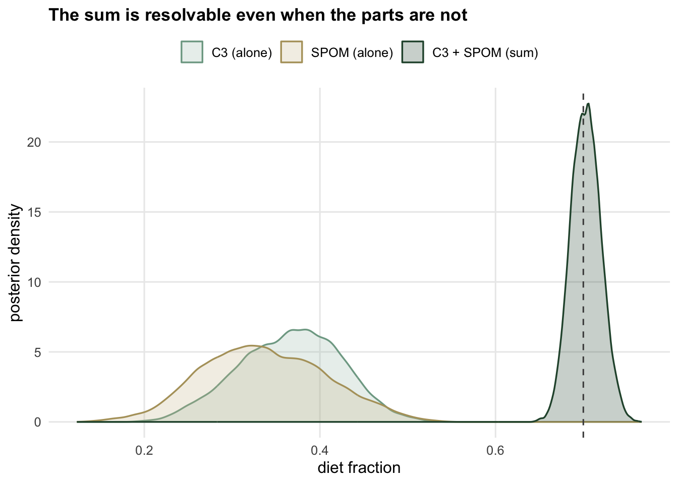
If the tracers fix the sum of the two depleted sources, then that sum is the quantity the data determine, even though neither source alone is. Add the posterior draws for C3 and SPOM (and, symmetrically, for the two enriched sources C4 and Algae) and the picture sharpens dramatically.

g_depleted <- d[, "C3"] + d[, "SPOM"]                    # true sum: 0.70
g_enriched <- d[, "C4"] + d[, "Algae"]                   # true sum: 0.30
summ <- function(z) c(mean(z), sd(z), as.numeric(quantile(z, c(0.025, 0.975))))
agg <- rbind(summ(g_depleted), summ(g_enriched))
dimnames(agg) <- list(c("C3 + SPOM", "C4 + Algae"), c("mean", "sd", "lo", "hi"))
sd_ind <- round(mean(apply(d, 2, sd)), 3)
sd_agg <- round(mean(c(sd(g_depleted), sd(g_enriched))), 3)
gain <- round(sd_ind / sd_agg, 1)
round(agg, 3)

            mean    sd    lo    hi
C3 + SPOM  0.703 0.019 0.667 0.739
C4 + Algae 0.297 0.019 0.261 0.333

c(individual_sd = sd_ind, aggregate_sd = sd_agg, narrower_by = gain)

individual_sd  aggregate_sd   narrower_by 
        0.071         0.019         3.700 

The depleted group sums to a posterior mean of 0.703 with a standard deviation of just 0.019, and its credible interval brackets the true 0.70 tightly. The individual sources had an average posterior standard deviation of 0.071; the grouped sum is 3.7 times narrower. The strong negative correlation that made the individuals ambiguous is exactly what makes their sum precise: the errors cancel. A mixing model that cannot tell C3 from SPOM can still tell you, with confidence, how much of the diet came from depleted sources as a whole.

Figure 4: The two individual depleted sources (wide, pale) against their sum (narrow, dark). Neither source alone is resolvable, but the quantity that matters ecologically, the total depleted contribution, is pinned down. Aggregating sources that trade off against each other turns an unanswerable question into an answerable one.

Does more data help?

If the width came from sampling noise, more consumer measurements would shrink it. Some of it does: raise the consumer sample from 20 to 200 and refit.

set.seed(505)
y4b <- cbind(rnorm(200, mu4[1], sd4[1]), rnorm(200, mu4[2], sd4[2]))
fit4b <- mix_mh(y4b, Smu, Ssd, res, iter = 60000, burn = 12000, seed = 606)
# one data set is one draw: repeat both sizes on fresh data, own seeds for each
n_rep <- 8
sd_fit <- function(draws) mean(apply(draws, 2, sd))
sd_rep <- function(nn, k) {
  set.seed(1000 + k)
  yy <- cbind(rnorm(nn, mu4[1], sd4[1]), rnorm(nn, mu4[2], sd4[2]))
  sd_fit(mix_mh(yy, Smu, Ssd, res, iter = 60000, burn = 12000, seed = 2000 + k)$draws)
}
sd20 <- c(sd_fit(d), sapply(1:(n_rep - 1), function(k) sd_rep(20, k)))
sd200 <- c(sd_fit(fit4b$draws), sapply(n_rep:(2 * n_rep - 2), function(k) sd_rep(200, k)))
sd_small <- round(mean(sd20), 3)
sd_large <- round(mean(sd200), 3)
ratio <- round(sd_large / sd_small, 2)
round(rbind(n20 = sd20, n200 = sd200), 3)

      [,1]  [,2]  [,3]  [,4]  [,5]  [,6]  [,7]  [,8]
n20  0.071 0.108 0.086 0.094 0.091 0.081 0.085 0.087
n200 0.047 0.050 0.053 0.082 0.072 0.060 0.051 0.077

c(sd_n20 = sd_small, sd_n200 = sd_large, ratio = ratio)

 sd_n20 sd_n200   ratio 
  0.088   0.062   0.700 

One data set of each size is a single draw, and the width it leaves varies a good deal from draw to draw, so the comparison is made over 8 simulated data sets of each size. Averaged over them, ten times as much data shrinks the individual standard deviations to 0.7 of their former size, short of the reduction to about a third that pure sampling noise would give (the square root of ten). Part of the uncertainty shrinks with data at the usual rate and part of it more slowly, but in this model the slower part is not a hard floor. The source spreads are treated as known, so the predicted variance depends on the diet, and that gives the data a handle on the direction the two tracer means cannot see; with enough consumers it narrows too. The handle comes from the variance assumption rather than from the isotope means, and it is only as trustworthy as that assumption. The aggregate was already tight at twenty measurements. The lesson is to spend effort where it pays: more tracers to break the geometric ambiguity, or grouping to report what is identifiable, rather than more consumer replicates, which can only resolve the remaining ambiguity through the assumed source spreads.

Where to go next

This posterior is only as trustworthy as its inputs. The source values here were corrected to the consumer’s trophic level before any fitting, and that correction, the trophic discrimination factor, turns out to move the answer more than the data do. Before reporting a fit, run the standard checks: is the consumer inside the mixing polygon, is the posterior actually informed by the data rather than the prior, and which contributions are resolvable as groups.

Honest limits

The sampler here is deliberately minimal: one consumer, fixed source means and spreads, a flat prior, and a hand-rolled Metropolis step. Production tools add hierarchical structure, covariates, informative priors, and better-mixing samplers, and you should use them for real analyses (SIAR, MixSIAR, and their relatives). What the toy version buys is transparency: the wide posterior and the strong correlations are not artefacts of a black box, they are the honest consequence of asking two tracers to resolve four sources. A fancier sampler would report the same width. The fix is more information, not more computation.

References

Moore JW, Semmens BX 2008 Ecology Letters 11:470-480 (10.1111/j.1461-0248.2008.01163.x).

Parnell AC, Inger R, Bearhop S, Jackson AL 2010 PLoS ONE 5:e9672 (10.1371/journal.pone.0009672).

Parnell AC, Phillips DL, Bearhop S, Semmens BX, Ward EJ, Moore JW, Jackson AL, Grey J, Kelley DJ, Inger R 2013 Environmetrics 24:387-399 (10.1002/env.2221).

Stock BC, Jackson AL, Ward EJ, Parnell AC, Phillips DL, Semmens BX 2018 PeerJ 6:e5096 (10.7717/peerj.5096).

Related tutorials

• Stable isotope mixing models in R
• Discrimination and concentration in mixing models
• Checking a stable isotope mixing model
• A Metropolis sampler from scratch

Reproducibility

• Code last run: 2026-10-15
• R version 4.5.3 (2026-03-11), aarch64-apple-darwin20
• Packages: ggplot2 4.0.3