library(ggplot2)

te_paper  <- "#f5f4ee"
te_ink    <- "#16241d"
te_body   <- "#2c3a31"
te_forest <- "#275139"
te_rust   <- "#b5534e"
te_gold   <- "#c9b458"
te_line   <- "#dad9ca"

theme_datasheet <- function() {
  theme_minimal(base_size = 12) +
    theme(plot.background  = element_rect(fill = te_paper, colour = NA),
          panel.background = element_rect(fill = te_paper, colour = NA),
          panel.grid.major = element_line(colour = te_line, linewidth = 0.3),
          panel.grid.minor = element_blank(),
          text             = element_text(colour = te_body),
          plot.title       = element_text(colour = te_ink, face = "bold"),
          plot.subtitle    = element_text(colour = te_body),
          axis.text        = element_text(colour = te_body))
}

mc_se  <- function(p, reps) sqrt(p * (1 - p) / reps)
covers <- function(ci, truth) truth >= ci[1] & truth <= ci[2]

cp_split <- function(gx, gy) {                 # least squares split point, one pass
  nn <- length(gy); o <- order(gx); xs <- gx[o]; cs <- cumsum(gy[o]); k <- 1:(nn - 1)
  kh <- which.max(cs[k]^2 / k + (cs[nn] - cs[k])^2 / (nn - k))
  (xs[kh] + xs[kh + 1]) / 2
}
sim_step <- function(nn, jump = 2, noise = 1) {
  gx <- runif(nn); list(x = gx, y = 10 + jump * (gx > 0.5) + rnorm(nn, 0, noise))
}
boot_draw <- function(est, gx, gy, mm, b_in)   # mm rows out of n, with replacement
  replicate(b_in, { i <- sample.int(length(gy), mm, TRUE); est(gx[i], gy[i]) })

n_survey <- 200; psi_true <- 0.5; depth_top <- 5; depth_span <- 40
set.seed(808)
survey    <- sim_step(n_survey); psi_hat <- cp_split(survey$x, survey$y)
ci_one    <- unname(quantile(boot_draw(cp_split, survey$x, survey$y, n_survey, 600),
                             c(0.025, 0.975)))
depth_hat <- depth_top + depth_span * psi_hat; depth_ci <- depth_top + depth_span * ci_oneThe m out of n bootstrap
R
bootstrap
resampling
statistics
ecology tutorial
Subsampling in R: why a step changepoint interval rests on the convergence rate exponent, how to fit that exponent, and where the repair does harm instead.
A benthic sled survey returns two hundred samples spread over forty metres of depth, from five metres down to forty five. The response is the wet biomass of a cold water amphipod per sample, and it does not change smoothly with depth. The animal is scarce in the warm surface layer and abundant below the thermocline, and the transition between the two levels happens over a distance shorter than the spacing of the samples. The report needs the depth of that transition, with an interval on it.
The estimator is a split point: run through every candidate depth, fit a two level mean, and keep the depth that minimises the residual sum of squares. A cumulative sum does the whole search in one pass. Threshold models of this kind are standard in ecology, and Toms and Lesperance set out the fitting side of them. The natural interval is a case bootstrap, which is what this site prescribes for the segmented regression breakpoint: resample rows, refit the whole procedure, collect the split point each time, and read off the percentiles.
Measured below, that interval falls short of its nominal 95 per cent, and the shortfall does not close as the survey grows. The repair is the m out of n bootstrap: refit on subsamples of size m much smaller than n, then rescale the resulting spread back to the full sample. This post measures what that rescaling costs and what it buys. The single number it turns on is the rate exponent, and the finding is that the exponent, not the subsample size, is the method: with the wrong exponent the same subsamples give an interval about three times too wide, or a coverage that collapses by half. The exponent does not have to be guessed, because it can be fitted from the subsamples that have already been drawn.
Two neighbouring posts set the boundaries. Checking a bootstrap ends on a diagnosis: if the statistic can jump, the bootstrap may be inconsistent, and simulating from a model or an exact result is the safer route. This post supplies the repair for the case where no exact result exists, and confirms below that where an exact result does exist it still wins. In the other direction, the case bootstrap that Segmented regression for a breakpoint runs is measured here as a control and comes out fine, because the continuous slope change breakpoint converges at a different rate from the step. The gap this post fills is narrow: it is the step model, which Checking a threshold model fits and never bootstraps.
A step in biomass, and an interval that looks fine
The gradient is rescaled to run from 0 to 1 so that widths read as fractions of the surveyed range, and the truth is placed at the midpoint. Nothing below depends on the direction of the step.
On this survey the split point sits at 0.494, which is 24.78 metres, against a truth of 25.00 metres. The case bootstrap interval runs from 24.44 to 25.96 metres, a width of 1.52 metres on a 40 metre transect. There is nothing visibly wrong with it. The rest of the post is about what that interval does over many surveys rather than one.
The split point converges faster than a regression slope
One piece of theory sits under everything below, and it is asserted rather than measured: an estimator has a rate tau_n such that tau_n * (theta_hat - theta) settles down to a fixed distribution as the sample grows, and for the estimators here that rate is a power, tau_n = n^beta. A sample mean or a regression slope has beta = 0.5. The published rate for a step changepoint with a fixed jump and a continuous covariate is n^1, worked out for this class of estimators by Dumbgen and going back to Hinkley for the sequence version of the problem; for isotonic type estimators read at a point it is n^(1/3). The exponent is also measurable, and that matters more here than the theory does, because it is what licenses fitting it later. Draw many data sets at each of several sample sizes, record the spread of the estimator, and regress log spread on log n. The slope is minus the exponent.
psi_grid <- seq(0.15, 0.85, length.out = 41)
kink_est <- function(gx, gy) {                 # continuous slope change breakpoint
  rss <- vapply(psi_grid, function(p)
    sum(.lm.fit(cbind(1, gx, pmax(gx - p, 0)), gy)$residuals^2), 0)
  psi_grid[which.min(rss)]
}
sim_kink <- function(nn, noise = 1) {
  gx <- runif(nn); list(x = gx, y = 1 + 0.2 * gx - 4 * pmax(gx - 0.5, 0) + rnorm(nn, 0, noise))
}
iso_at <- function(gx, gy, x0 = 0.5) {         # monotone fit, read at an interior point
  o <- order(gx); xs <- gx[o]; yf <- -isoreg(xs, -gy[o])$yf
  yf[max(1, sum(xs <= x0))]
}
sim_iso <- function(nn, noise = 1) {
  gx <- runif(nn); list(x = gx, y = 2 - 2 * gx + rnorm(nn, 0, noise))
}
loglog_beta <- function(spread, sizes) -unname(coef(lm(log(spread) ~ log(sizes)))[2])
loglog_se   <- function(spread, sizes) coef(summary(lm(log(spread) ~ log(sizes))))[2, 2]
spread_by_n <- function(gen, est, sizes, reps)
  sapply(sizes, function(nn) sd(replicate(reps, { d <- gen(nn); est(d$x, d$y) })))

r_rate <- 1500
n_rate <- c(50, 100, 200, 400, 800, 1600)
n_kink <- c(100, 200, 400, 800, 1600)
set.seed(1);   sd_step <- spread_by_n(sim_step, cp_split, n_rate, r_rate)
set.seed(121); sd_kink <- spread_by_n(sim_kink, kink_est, n_kink, r_rate)
set.seed(101); sd_iso  <- spread_by_n(sim_iso,  iso_at,   n_rate[-1], r_rate)
beta_step <- loglog_beta(sd_step, n_rate); se_step <- loglog_se(sd_step, n_rate)
beta_kink <- loglog_beta(sd_kink, n_kink); se_kink <- loglog_se(sd_kink, n_kink)
beta_iso  <- loglog_beta(sd_iso, n_rate[-1]); se_iso <- loglog_se(sd_iso, n_rate[-1])
n_fold    <- n_rate[length(n_rate)] / n_rate[1]
sd_fold   <- sd_step[1] / sd_step[length(n_rate)]
Over 1500 data sets per sample size, the standard deviation of the split point falls from 0.0379 at n = 50 to 0.00119 at n = 1600, an exponent of 1.010 with a standard error of 0.013 from the log log fit. Multiplying the sample by 32 divides the spread by 32, where a square root rate would have divided it by 5.7. The continuous slope change breakpoint, fitted on the same scaled gradient, comes out at 0.618 (standard error 0.017), much closer to the square root rate than to the split point’s, and the monotone fit read at an interior point at 0.334 (standard error 0.011), near a third. A step changepoint is often filed under cube root asymptotics; it is not. It converges at n^1, faster than anything regular, and the estimator with a genuine cube root rate is the monotone fit, which turns up later as a case where the repair does harm.
The shortfall does not close with more data
The percentile bootstrap for the split point is run next at three sample sizes, alongside the basic (reversed) interval, and against an oracle width taken from direct draws of the estimator. The same case bootstrap is then run on the continuous breakpoint as a control.
r_cov <- 400; b_in <- 250
set.seed(21)
cov_tab <- do.call(rbind, lapply(c(100, 200, 400), function(nn) {
  oracle <- unname(diff(quantile(replicate(3000, { d <- sim_step(nn); cp_split(d$x, d$y) }),
                                 c(0.025, 0.975))))
  hit_p <- hit_b <- wsum <- 0
  for (r in 1:r_cov) {
    d <- sim_step(nn); ph <- cp_split(d$x, d$y)
    q <- unname(quantile(boot_draw(cp_split, d$x, d$y, nn, b_in), c(0.025, 0.975)))
    hit_p <- hit_p + covers(q, psi_true); wsum <- wsum + (q[2] - q[1])
    hit_b <- hit_b + covers(2 * ph - rev(q), psi_true)
  }
  data.frame(n = nn, oracle = oracle, pct = hit_p / r_cov,
             basic = hit_b / r_cov, width = wsum / r_cov)
}))
cov_tab$ratio <- cov_tab$width / cov_tab$oracle; cov_se <- mc_se(cov_tab$pct, r_cov)

r_ctl <- 250; b_ctl <- 200
set.seed(122)
ctl_tab <- do.call(rbind, lapply(c(120, 400), function(nn) {
  hit <- wsum <- 0
  for (r in 1:r_ctl) {
    d <- sim_kink(nn)
    q <- unname(quantile(boot_draw(kink_est, d$x, d$y, nn, b_ctl), c(0.025, 0.975)))
    hit <- hit + covers(q, psi_true); wsum <- wsum + (q[2] - q[1])
  }
  data.frame(n = nn, cov = hit / r_ctl, width = wsum / r_ctl)
}))
ctl_se <- mc_se(ctl_tab$cov, r_ctl)
Across 400 surveys per sample size, each with 250 resamples, the percentile interval covers 0.915, 0.900 and 0.912 at n = 100, 200 and 400, with a Monte Carlo standard error near 0.015. Quadrupling the survey does not move it. That flatness is the whole problem: an interval that is a little short at the smallest of those sizes and still a little short at the largest is not suffering from a small sample, it is converging to the wrong answer. The basic interval, built from the same resamples, covers between 0.810 and 0.848, and the disagreement between two intervals read off one bootstrap distribution is itself a warning sign. The width is not the fault: the percentile interval runs between 1.07 and 1.17 times the oracle width, the width the estimator’s own sampling distribution deserves. An interval that is slightly wide and still under covers is mis-shaped, not mis-scaled.
cov_long <- rbind(
  data.frame(n = cov_tab$n, cov = cov_tab$pct,   arm = "step model, percentile"),
  data.frame(n = cov_tab$n, cov = cov_tab$basic, arm = "step model, basic"),
  data.frame(n = ctl_tab$n, cov = ctl_tab$cov,   arm = "continuous breakpoint (control)"))
cov_long$arm <- factor(cov_long$arm, levels = c("continuous breakpoint (control)",
                                                "step model, percentile", "step model, basic"))

ggplot(cov_long, aes(n, cov, colour = arm)) +
  geom_hline(yintercept = 0.95, linetype = "dashed", colour = te_ink, linewidth = 0.6) +
  geom_line(linewidth = 0.9) + geom_point(size = 2.6) +
  scale_x_log10(breaks = c(100, 120, 200, 400)) +
  scale_colour_manual(values = c(te_forest, te_rust, te_gold), name = NULL) +
  scale_y_continuous(limits = c(0.75, 1)) +
  labs(x = "sample size", y = "coverage of a nominal 95 per cent interval",
       title = "More data does not repair it", subtitle = "dashed line: nominal 0.95") +
  theme_datasheet() + theme(legend.position = "bottom")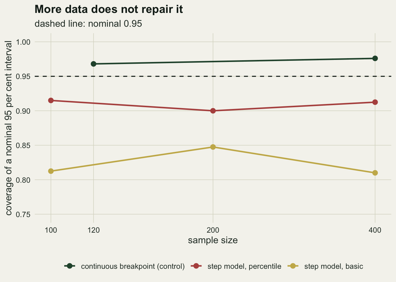
The control is the part of that figure to read first. On the continuous slope change breakpoint the same case bootstrap covers 0.968 at n = 120 and 0.976 at n = 400, with a standard error near 0.011: at or above the nominal level, never below it. The advice in the segmented regression post is sound for the model that post fits. The failure belongs to the step, and the reason is the exponent measured above.
The exponent, not the subsample size, sets the interval
Here is the algebra, which is arithmetic rather than a finding, and which is the argument Politis and Romano set out for subsampling in general. If tau_n * (psi_hat - psi) has a limit distribution, then subsamples of size m give a copy of that limit at rate tau_m, centred on psi_hat instead of on psi. Solving the pivot for psi gives
CI = psi_hat - (m / n)^beta * quantile(psi_star - psi_hat, c(0.975, 0.025))
where psi_star are the subsample estimates. The factor (m / n)^beta is the whole method. Since m is smaller than n that factor is below one, and it shrinks faster the larger beta is, so taking beta = 0.5 when the truth is 1 inflates every interval by the square root of n over m. The consistency requirement is theory as well: m must grow with n while m over n goes to zero. What the choice costs is measurement, and the sweep below holds the sample at the size of the example survey, 200, and runs m from about n^0.4 to n^0.9, building two intervals from each set of subsamples: one with the rate exponent, one with the square root convention a reader would carry over from an ordinary bootstrap.
rescale_ci <- function(ph, dev, mm, nn, bexp)  # the m out of n interval
  unname(ph - (mm / nn)^bexp * quantile(dev, c(0.975, 0.025)))

r_swp <- 400; b_swp <- 250; n_swp <- n_survey
set.seed(31)
m_swp <- unique(round(n_swp^c(0.4, 0.5, 0.6, 0.7, 0.8, 0.9)))
acc <- wid <- matrix(0, length(m_swp), 2)
for (r in 1:r_swp) {
  d <- sim_step(n_swp); ph <- cp_split(d$x, d$y)
  for (j in seq_along(m_swp)) {
    dev <- boot_draw(cp_split, d$x, d$y, m_swp[j], b_swp) - ph
    for (bj in 1:2) {
      ci <- rescale_ci(ph, dev, m_swp[j], n_swp, c(1, 0.5)[bj])
      acc[j, bj] <- acc[j, bj] + covers(ci, psi_true)
      wid[j, bj] <- wid[j, bj] + (ci[2] - ci[1])
    }
  }
}
swp <- data.frame(m = m_swp, frac = m_swp / n_swp,
                  cov_rate = acc[, 1] / r_swp, w_rate = wid[, 1] / r_swp,
                  cov_sqrt = acc[, 2] / r_swp, w_sqrt = wid[, 2] / r_swp)
oracle_swp <- cov_tab$oracle[cov_tab$n == n_swp]
best_j <- which.max(swp$cov_rate); mid_j <- which(swp$m == round(n_swp^0.6))
gap_width <- swp$w_sqrt[mid_j] / swp$w_rate[mid_j]
With the rate exponent, coverage is a hump in m: 0.902 at m = 8, a peak of 0.938 at m = 14, and 0.885 at m = 118. Best to worst across that whole sweep is 0.052. With the square root convention on the same subsamples, coverage at m = 24 is 0.993, an interval that almost never misses because at that same subsample size it is 2.9 times wider than the rate exponent interval, against an oracle width of 0.0397. Choosing m badly moves coverage across the span just given. Choosing the exponent badly costs that factor of three in width.
swp_long <- data.frame(frac = rep(swp$frac, 4),
  y     = c(swp$cov_rate, swp$cov_sqrt, swp$w_rate, swp$w_sqrt),
  panel = rep(c("coverage", "interval width"), each = 2 * nrow(swp)),
  rescaling = rep(rep(c("rate exponent", "square root"), each = nrow(swp)), 2))
ref_line <- data.frame(panel = c("coverage", "interval width"), y = c(0.95, oracle_swp))

ggplot(swp_long, aes(frac, y, colour = rescaling)) +
  geom_hline(data = ref_line, aes(yintercept = y),
             linetype = "dashed", colour = te_ink, linewidth = 0.6) +
  geom_line(linewidth = 0.9) + geom_point(size = 2.2) +
  facet_wrap(~ panel, scales = "free_y") +
  scale_x_log10() +
  scale_colour_manual(values = c(te_forest, te_rust), name = NULL) +
  labs(x = "subsample fraction m / n", y = NULL,
       title = "The exponent moves the interval, not the subsample size",
       subtitle = "dashed: nominal 0.95 on the left, the oracle width on the right") +
  theme_datasheet() + theme(legend.position = "bottom", strip.text = element_text(colour = te_ink))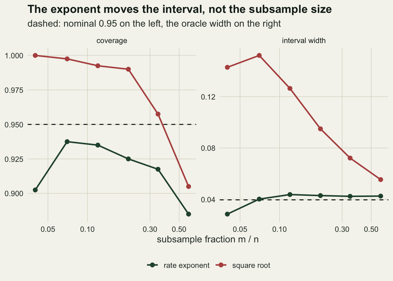
The exponent can be fitted from the subsamples you already drew
The objection to all of this is that a field ecologist does not know beta. The objection has a measured answer, and it costs no extra fieldwork. The spread of the subsample distribution scales as m^(-beta), so drawing that distribution over a geometric grid of m and regressing log spread on log m returns the exponent as minus the slope. The interval itself needs subsamples at a single m, so every other m on the grid is drawn for the fit alone: the exponent is paid for in resampling time, not in data.
fit_run <- function(nn, jump, seed, adaptive = FALSE, r_fit = 400, b_fit = 250) {
  set.seed(seed)
  mg    <- unique(round(nn * 0.7^(1:6)))
  jstar <- which.min(abs(mg - round(nn^0.6)))
  bhat  <- m_vol <- numeric(r_fit)
  hit   <- wid <- c(ord = 0, known = 0, fitted = 0, sq = 0, vol = 0)
  add   <- function(nm, ci) {
    hit[nm] <<- hit[nm] + covers(ci, psi_true); wid[nm] <<- wid[nm] + (ci[2] - ci[1])
  }
  for (r in 1:r_fit) {
    d <- sim_step(nn, jump = jump); ph <- cp_split(d$x, d$y)
    add("ord", unname(quantile(boot_draw(cp_split, d$x, d$y, nn, b_fit), c(0.025, 0.975))))
    dev <- lapply(mg, function(mm) boot_draw(cp_split, d$x, d$y, mm, b_fit) - ph)
    spread <- sapply(dev, function(v) unname(diff(quantile(v, c(0.1, 0.9)))))
    bh <- loglog_beta(spread, mg); bhat[r] <- bh
    mk <- function(j, bexp) rescale_ci(ph, dev[[j]], mg[j], nn, bexp)
    add("fitted", mk(jstar, bh)); add("known", mk(jstar, 1)); add("sq", mk(jstar, 0.5))
    if (adaptive) {
      ends <- t(sapply(seq_along(mg), function(j) mk(j, bh)))
      vol  <- sapply(2:(length(mg) - 1), function(j)
        sd(ends[(j - 1):(j + 1), 1]) + sd(ends[(j - 1):(j + 1), 2]))
      jv <- which.min(vol) + 1; m_vol[r] <- mg[jv]; add("vol", ends[jv, ])
    }
  }
  c(list(n = nn, m = mg[jstar], reps = r_fit, b = b_fit, bhat = bhat, m_vol = median(m_vol)),
    as.list(hit / r_fit), setNames(as.list(wid / r_fit), paste0("w_", names(wid))))
}
fit200 <- fit_run(200, 2, 61, adaptive = TRUE)
fit400 <- fit_run(400, 4, 131)
At n = 200 with a step of two residual standard deviations, the fitted exponent averages 1.022 with a standard deviation of 0.390 across 400 surveys, against a truth of one. The interval built on the fitted exponent covers 0.907, against 0.915 when the exponent is handed to it and 0.890 for the ordinary bootstrap. Fitting is free here, in the sense that the difference between it and knowing the truth is smaller than the Monte Carlo error of either. The square root convention on the same subsamples covers 0.990 at 2.9 times the width.
ggplot(data.frame(b = fit400$bhat), aes(b)) +
  geom_histogram(bins = 30, fill = te_forest, colour = te_paper, linewidth = 0.2) +
  geom_vline(xintercept = 1, linetype = "dashed", colour = te_rust, linewidth = 0.8) +
  labs(x = "fitted exponent", y = "surveys",
       title = paste("One exponent per survey, over", fit400$reps, "surveys"),
       subtitle = "dashed red: the true exponent") + theme_datasheet()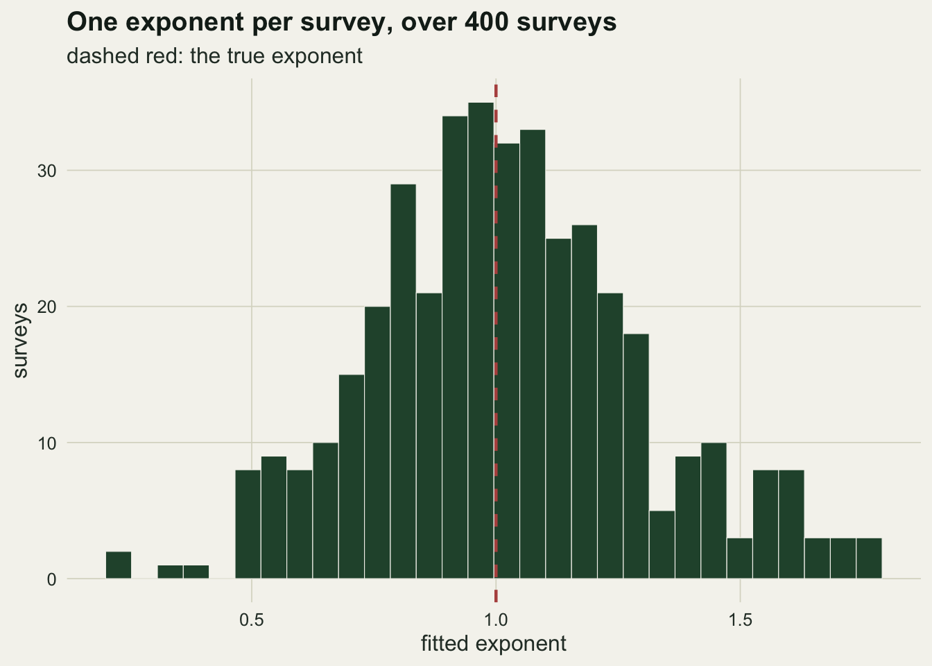
The histogram is what the estimate does over many surveys, and its spread is not small: at n = 400 with the sharpest step tested the fitted exponent averages 1.021 with a standard deviation of 0.278. That spread is the price. In this setting the ordinary bootstrap covers 0.875, the known exponent lifts it to 0.948 at a width of 0.0082 against 0.0083, and the fitted exponent reaches 0.902, part of the way back. Those two widths are the same to the resolution of this study, so the coverage the known exponent buys here costs nothing measurable in width.
A published rule for choosing m from the data was run on the same subsamples at n = 200, using the fitted exponent. The minimum volatility rule of Politis, Romano and Wolf picks the m at which the interval endpoints are most stable across neighbouring m, and covers 0.873 at a median m of 69, against 0.907 for the fixed choice m = round(n^0.6), which here is m = 24. Choosing m per data set does not improve on the fixed choice.
A repair for under-coverage, not a general upgrade
No run so far has varied the step size at a fixed sample size. The next question is what the headline depends on, and the answer is not sample size.
r_grd <- 400; b_grd <- 250
set.seed(81)
cells <- expand.grid(n = c(100, 400), snr = c(1, 2, 4))
cell_tab <- do.call(rbind, lapply(seq_len(nrow(cells)), function(g) {
  nn <- cells$n[g]; mm <- round(nn^0.6); h_ord <- h_mofn <- 0
  for (r in 1:r_grd) {
    d <- sim_step(nn, jump = cells$snr[g]); ph <- cp_split(d$x, d$y)
    q <- unname(quantile(boot_draw(cp_split, d$x, d$y, nn, b_grd), c(0.025, 0.975)))
    h_ord <- h_ord + covers(q, psi_true)
    dev <- boot_draw(cp_split, d$x, d$y, mm, b_grd) - ph
    h_mofn <- h_mofn + covers(rescale_ci(ph, dev, mm, nn, 1), psi_true)
  }
  data.frame(n = nn, snr = cells$snr[g], m = mm, ord = h_ord / r_grd, mofn = h_mofn / r_grd)
}))
pick <- function(nn, ss) cell_tab[cell_tab$n == nn & cell_tab$snr == ss, ]
weak <- pick(100, 1); sharp <- pick(400, 4); mid <- pick(400, 2)
grd_se <- mc_se(0.9, r_grd); grd_dse <- sqrt(2) * grd_se
Quadrupling the sample at a sharp step, from n = 100 to n = 400, takes the ordinary bootstrap from 0.875 to 0.845: no repair, and if anything a little worse. Moving the step from one residual standard deviation to four at n = 400 moves it from 0.963 to 0.845. The sharper the step, the worse the ordinary bootstrap, because the sharper the step the more the estimator behaves like the discrete object it is. The sign of the repair flips with it: at a sharp step the m out of n interval lifts coverage to 0.932, while at a step of one residual standard deviation with n = 100 it drops coverage from 0.973 to 0.772. The standard error of a difference between two coverages measured over 400 surveys each is about 0.021, so that drop is real many times over. The other end of the question is what the method costs on an estimator that never needed it, and the regression slope is the reference case: smooth, root n, the bootstrap’s home ground.
lin_slope <- function(gx, gy) unname(coef(.lm.fit(cbind(1, gx), gy))[2])
r_reg <- 600; b_reg <- 250; n_reg <- 200; b_true <- 2
set.seed(41)
m_reg <- unique(round(n_reg^c(0.5, 0.6, 0.7, 0.8, 0.9)))
h_ord <- w_ord <- 0; h_sq <- w_sq <- h_wrong <- numeric(length(m_reg))
for (r in 1:r_reg) {
  gx <- runif(n_reg); gy <- 1 + b_true * gx + rnorm(n_reg); th <- lin_slope(gx, gy)
  q  <- unname(quantile(boot_draw(lin_slope, gx, gy, n_reg, b_reg), c(0.025, 0.975)))
  h_ord <- h_ord + covers(q, b_true); w_ord <- w_ord + (q[2] - q[1])
  for (j in seq_along(m_reg)) {
    dev <- boot_draw(lin_slope, gx, gy, m_reg[j], b_reg) - th
    ci  <- rescale_ci(th, dev, m_reg[j], n_reg, 0.5)
    h_sq[j] <- h_sq[j] + covers(ci, b_true); w_sq[j] <- w_sq[j] + (ci[2] - ci[1])
    h_wrong[j] <- h_wrong[j] + covers(rescale_ci(th, dev, m_reg[j], n_reg, 1), b_true)
  }
}
reg_ord <- h_ord / r_reg
reg_tab <- data.frame(m = m_reg, cov_sq = h_sq / r_reg, cov_wrong = h_wrong / r_reg,
                      inflation = (w_sq / r_reg) / (w_ord / r_reg))
reg_mid <- reg_tab[reg_tab$m == round(n_reg^0.6), ]
Run with the correct exponent for a slope, which is one half, the m out of n interval covers between 0.948 and 0.963 across the whole sweep against 0.943 for the ordinary bootstrap, and pays between 0 and 8 per cent in width. That is the cost of applying it where it was not needed: small, and paid in width rather than in coverage.
Carrying the changepoint exponent over to the slope is another matter. The same subsamples, rescaled by m over n instead of by its square root, cover 0.408 at m = 14 and 0.852 at the largest m: a 54 point loss of coverage, from a rescaling that looks like a detail in the code.
The last case is the one the method was invented for. A monotone fit read at an interior point has cube root asymptotics, and Sen, Banerjee and Woodroofe proved the ordinary bootstrap inconsistent for it, so this is where a rescaled subsample interval should be at its best.
r_iso <- 1000; b_iso <- 200; n_iso2 <- 200; mu_true <- 1
set.seed(111)
mg_iso <- unique(round(n_iso2 * 0.7^(1:6)))
j_iso  <- which.min(abs(mg_iso - round(n_iso2^0.6)))
bhat_iso <- numeric(r_iso); h_iso <- c(ord = 0, third = 0, sq = 0, fitted = 0)
for (r in 1:r_iso) {
  d <- sim_iso(n_iso2); th <- iso_at(d$x, d$y)
  q <- unname(quantile(boot_draw(iso_at, d$x, d$y, n_iso2, b_iso), c(0.025, 0.975)))
  h_iso["ord"] <- h_iso["ord"] + covers(q, mu_true)
  dev <- lapply(mg_iso, function(mm) boot_draw(iso_at, d$x, d$y, mm, b_iso) - th)
  spread <- sapply(dev, function(v) unname(diff(quantile(v, c(0.1, 0.9)))))
  bh <- loglog_beta(spread, mg_iso); bhat_iso[r] <- bh
  mk_iso <- function(bexp) rescale_ci(th, dev[[j_iso]], mg_iso[j_iso], n_iso2, bexp)
  h_iso["third"]  <- h_iso["third"]  + covers(mk_iso(1 / 3), mu_true)
  h_iso["sq"]     <- h_iso["sq"]     + covers(mk_iso(0.5),   mu_true)
  h_iso["fitted"] <- h_iso["fitted"] + covers(mk_iso(bh),    mu_true)
}
h_iso <- h_iso / r_iso; iso_se <- mc_se(h_iso[["ord"]], r_iso)

# reference case only: the maximum of a uniform sample, owned by two earlier posts
# run at high replication because the gap it has to resolve is a couple of points
r_umx <- 4000; b_umx <- 300; n_umx <- 40; m_umx <- round(n_umx^0.7)
set.seed(51)
h_mm <- w_mm <- 0
for (r in 1:r_umx) {
  xv  <- runif(n_umx); th <- max(xv)
  dev <- replicate(b_umx, max(sample(xv, m_umx, TRUE))) - th
  ci  <- rescale_ci(th, dev, m_umx, n_umx, 1)
  h_mm <- h_mm + covers(ci, 1); w_mm <- w_mm + (ci[2] - ci[1])
}
umx_cov <- h_mm / r_umx; umx_wid <- w_mm / r_umx; umx_se <- mc_se(umx_cov, r_umx)
nominal <- 0.95
umx_short <- nominal - umx_cov; umx_z <- umx_short / umx_se
set.seed(52); r_exact <- 3000
exact     <- replicate(r_exact, { xv <- runif(n_umx); c(max(xv), max(xv) / 0.05^(1 / n_umx)) })
umx_exact <- mean(exact[1, ] <= 1 & exact[2, ] >= 1); w_exact <- mean(exact[2, ] - exact[1, ])
reps_all  <- c(r_cov, r_ctl, r_swp, r_grd, fit200$reps, r_reg, r_iso, r_umx, r_exact)
b_all     <- c(b_in, b_ctl, b_swp, b_grd, fit200$b, b_reg, b_iso, b_umx)
The fitted exponent moves the right way here too: 0.389 on average with a standard deviation of 0.081, against a truth of one third. It sits above that truth by more than the Monte Carlo error of the average, so the fit is biased upwards at this sample size rather than exact. It still lands nowhere near the exponent the same procedure returned for the step model, which is the evidence that the fitting step is doing something real rather than returning whatever it was told. The intervals are another story. At n = 200 the ordinary bootstrap covers 0.951 with a standard error of 0.007, the correctly rescaled m out of n interval covers 0.857, the fitted one 0.812 and the square root one 0.716. The textbook success case is a harm case at a sample size an ecologist would recognise.
dumb <- data.frame(
  setting = c("sharp step, n = 400", "moderate step, n = 400", "weak step, n = 100",
              "monotone fit at a point, n = 200", "regression slope, wrong exponent"),
  before  = c(sharp$ord, mid$ord, weak$ord, h_iso[["ord"]], reg_ord),
  after   = c(sharp$mofn, mid$mofn, weak$mofn, h_iso[["third"]], reg_mid$cov_wrong))
dumb$setting <- factor(dumb$setting, levels = rev(dumb$setting))
dumb$better <- abs(dumb$after - 0.95) < abs(dumb$before - 0.95)

ggplot(dumb, aes(y = setting)) +
  geom_vline(xintercept = 0.95, linetype = "dashed", colour = te_ink, linewidth = 0.6) +
  geom_segment(aes(x = before, xend = after, yend = setting, colour = better),
               linewidth = 1.1, arrow = arrow(length = unit(0.11, "inches"), type = "closed")) +
  geom_point(aes(x = before), size = 2.8, shape = 21, fill = te_paper, colour = te_body) +
  scale_colour_manual(values = c(te_rust, te_forest), guide = "none") +
  scale_x_continuous(limits = c(0.45, 1.02)) +
  labs(x = "coverage of a nominal 95 per cent interval", y = NULL,
       title = "Where the repair helps and where it hurts",
       subtitle = "hollow point: ordinary bootstrap; arrow head: m out of n") + theme_datasheet()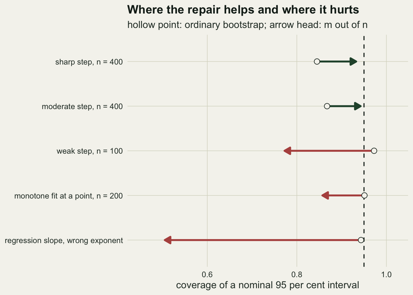
One case is deliberately left out of that figure, because two other posts own it: the maximum of a uniform sample, the standard demonstration that the bootstrap can fail outright, worked through in Checking a bootstrap and in Bootstrap confidence intervals. The ordinary bootstrap covers essentially nothing there, which is the point those two posts make. Rescaled subsamples lift it most of the way back and no further. Over 4000 samples at n = 40 and m = 13, run at that replication because the gap to be resolved is small, the m out of n interval covers 0.925 with a Monte Carlo standard error of 0.004: a shortfall of 0.025 below the nominal level, 6.0 standard errors of it, so the arm is under covering rather than drawing badly. That shortfall is what pays for the width. The subsample interval is the narrower of the two, 0.0732 against 0.0759, and it is narrower because it misses more often; the exact interval’s 95 per cent is exact by construction, and over 3000 draws it measures 0.951. On the one example here where an exact answer exists the subsample interval is beaten by it, which is why that post’s advice holds: when an exact result exists, take it, and reach for subsampling when none does.
What to report
Report the exponent you used and where it came from. An m out of n interval without its exponent is not reproducible, because the same subsamples support intervals that differ by a factor of three. If the exponent was fitted, give its estimate and its spread, and give the grid of m it was fitted over.
Report the subsample size and how it was chosen. A fixed m = round(n^0.6) is defensible, and the data driven rule tested here did not improve on it. If a data driven rule was used instead, say which, because it changes m from survey to survey and that variation has a cost.
Report the ordinary bootstrap alongside it. The decision to subsample is a claim that the ordinary interval under covers, and a reader cannot check that claim without seeing both. If the two agree, the choice did not matter, and saying so is cheap.
Say which model produced the estimator, and give the replication of any coverage study quoted. The step model and the continuous slope change model are different estimators of what a field report calls the same threshold, they converge at different rates, and only one of them needs any of this. Every coverage above is a proportion out of 250 to 4000 simulated surveys. Most of them run at 400, where the standard error of a gap between two coverages is about 0.021, so at that replication a gap under about 0.04 is not a gap. The arms that run at higher replication resolve smaller ones: the uniform maximum above is run over 4000 samples, where its 0.025 shortfall is 6.0 standard errors, and the monotone fit over 1000.
Honest limits
The repair makes things worse when the step is weak. At a step of one residual standard deviation with n = 100 the ordinary bootstrap covers 0.973 and the m out of n interval covers 0.772. That is the common regime in the field, the one where the threshold is not yet obvious, and it is exactly where the method should not be reached for. Nothing in the output of a single fit tells you which regime you are in: reading the step to noise ratio off the fit requires already believing the fit.
The estimator with genuine cube root asymptotics is a harm case at these sample sizes rather than a success case. The monotone fit at a point is the textbook motivation for the m out of n bootstrap, and over 1000 surveys at n = 200 the ordinary bootstrap sits at 0.951 with a standard error of 0.007, which is not below the nominal level. Asymptotic inconsistency is a statement about the limit, and at this sample size it leaves nothing that a practitioner would notice or mind. Every rescaled interval turns an interval that was already fine into an under-covering one, the best of them reaching only 0.857.
The fitted exponent is not free where the failure is worst. At n = 400 with the sharpest step it recovers 0.902 against 0.948 for the known exponent and 0.875 for the ordinary bootstrap. It closes part of that gap, but not a fraction this replication can pin down, because the fraction is a ratio of two differences and each of them carries its own Monte Carlo error. The estimate itself is good; the interval is a nonlinear function of it, and the spread of the estimate propagates asymmetrically. The log log fit also needs the grid of m to sit where the spread has not saturated, and at small n that range is short.
The whole study is one generating model, and the measured rates carry their own approximations. The response is Gaussian around two levels with a covariate uniform on the gradient, no spatial correlation, no zero inflation, no error in the recorded depth, and the truth at the midpoint of the range. The continuous breakpoint is fitted over a grid of 41 candidate positions rather than continuously, and its exponent is a log log slope through 5 points, each of them a standard deviation over 1500 draws; with a standard error of 0.017 on that slope, 0.618 says the estimator is far from the split point’s rate, not that its exponent is exactly that number. Counts, or a threshold near the end of a transect, or samples clustered by station, would each change the numbers, and clustering in particular would move the resampling to the station level.
The replication is set by the render budget. Every coverage above is a nested loop of surveys by resamples, with the inner count held between 200 and 300, which is a convention for reading a far tail quantile off a resample distribution rather than a tuned optimum. Not every comparison above is separated by its own Monte Carlo error. The ones that are: the ordinary bootstrap’s shortfall at a sharp step, the factor of three in width between the two rescalings, the coverage the wrong exponent costs on a regression slope, the drop the repair causes on a weak step, and the subsample interval’s shortfall on the uniform maximum, which is the one arm raised to 4000 surveys because the shortfall it had to resolve is only a couple of points. The ones that are not are never leaned on: fitting the exponent against knowing it at n = 200 is called a tie, the volatility rule is credited only with failing to improve on the fixed m, and the two widths at n = 400 are called equal.
References
Politis DN, Romano JP 1994 Annals of Statistics 22(4):2031-2050 (10.1214/aos/1176325770)
Politis DN, Romano JP, Wolf M 1999 Subsampling (ISBN 978-0-387-98854-2)
Sen B, Banerjee M, Woodroofe M 2010 Annals of Statistics 38(4):1953-1977 (10.1214/09-AOS777)
Dumbgen L 1991 Annals of Statistics 19(3):1471-1495 (10.1214/aos/1176348257)
Hinkley DV 1970 Biometrika 57(1):1-17 (10.1093/biomet/57.1.1)
Toms JD, Lesperance ML 2003 Ecology 84(8):2034-2041 (10.1890/02-0472)