library(ggplot2)
library(patchwork)

te_paper  <- "#f5f4ee"
te_ink    <- "#16241d"
te_body   <- "#2c3a31"
te_forest <- "#275139"
te_rust   <- "#b5534e"
te_gold   <- "#c9b458"
te_line   <- "#dad9ca"

theme_datasheet <- function() {
  theme_minimal(base_size = 12) +
    theme(plot.background  = element_rect(fill = te_paper, colour = NA),
          panel.background = element_rect(fill = te_paper, colour = NA),
          panel.grid.major = element_line(colour = te_line, linewidth = 0.3),
          panel.grid.minor = element_blank(),
          text             = element_text(colour = te_body),
          plot.title       = element_text(colour = te_ink, face = "bold"),
          plot.subtitle    = element_text(colour = te_body),
          axis.text        = element_text(colour = te_body))
}Species synchrony and community stability
R
community ecology
stability
synchrony
simulation
ecology tutorial
The Loreau-de Mazancourt synchrony index splits community variability exactly. Simulating in R how synchrony and mean-variance scaling set the diversity slope.
A long-term grassland experiment has clipped the same plots every summer for thirty years. The plots sown with sixteen species give a total biomass that wobbles less from year to year than the plots sown with two, and the wobble is summarised as the coefficient of variation of the plot total. The usual sentence in the results is that diversity stabilises the community. The sentence is true of the numbers, but it merges two separate pieces of arithmetic, and they respond to different things.
One piece is how the species move relative to each other. If a wet year that favours one grass also suppresses another, the total is steadier than either species. If every species tracks the same rainfall, adding species does nothing to damp the fluctuation of the total. The other piece is how the variance of one species relates to its own mean. Split a fixed total among more species and each one gets a smaller mean; whether a smaller population is proportionally noisier depends on the exponent of the mean-variance relationship.
The second piece has already been stated here. The post on biodiversity and ecosystem function closes on it: where sd = c * mu^(z/2), a stability ratio goes as mu^(1 - z/2), and “the arithmetic hands out a free gain only while the exponent z stays below two”. That paragraph concerns a mixture whose total mean is larger than the monoculture’s. The post on Taylor’s power law fits the same exponent across quadrats in space. What neither post contains is a measure of the first piece, the synchrony between species, and a way to separate it from the second. Loreau and de Mazancourt (2008) supplied one: a synchrony index, written here as phi, that sits between zero and one and enters community variability as an exact factor.
This is not the stability of a MAR(1) model, whose variance ratio is the share of stationary variance due to environmental noise; that quantity comes from a fitted MAR(1) model (its interaction matrix and its noise covariance), while phi is read off the raw abundance series with no model at all. Nor is it synchrony between populations of one species at different sites. Everything below stays inside one community, at one place, through time.
The synchrony index and an exact split
For species abundances observed over a run of years, write sigma_T for the standard deviation of the community total and sigma_i for the standard deviation of species i. Loreau and de Mazancourt define the synchrony index as
phi = sigma_T^2 / (sigma_1 + sigma_2 + ... + sigma_S)^2
The upper bound of one follows because the standard deviation of a sum can never exceed the sum of the standard deviations; it is reached only when every pair of species is perfectly positively correlated. The lower bound of zero is a community whose total does not vary at all while its species do. Rearranging the definition gives the split used by Loreau and de Mazancourt (2013):
CV_com = sqrt(phi) * sum_i (mu_i / mu_T) * CV_i = sqrt(phi) * (sum_i sigma_i) / mu_T
Community variability is the square root of synchrony times the abundance-weighted mean of the species coefficients of variation. There is nothing approximate in it. It holds for the sample moments of any data set, provided the variances and the standard deviations share a denominator, which var() and sd() in R do.
The simulation uses Gaussian abundances with a chosen mean for each species, a standard deviation set by a temporal mean-variance law sd_i = c * mu_i^(z/2), and a common correlation between every pair of species. All design constants are fixed here, before any run.
mu_tot  <- 100      # expected community total, held fixed throughout
c_tay   <- 0.4      # coefficient of the mean-variance law
z_main  <- 1.5      # exponent used unless stated otherwise
n_year  <- 30       # length of each series
n_rep   <- 400      # simulated communities per design point
n_batch <- 10       # batches for Monte Carlo standard errors
S_grid  <- c(2, 3, 4, 6, 8, 12, 16, 24, 32, 40)

sync_phi <- function(abund) {
  var(rowSums(abund)) / sum(apply(abund, 2, sd))^2
}
cv_total <- function(abund) sd(rowSums(abund)) / mean(rowSums(abund))

# n_year by S matrix of abundances with equal pairwise correlation rho
sim_comm <- function(mu_sp, rho, z, n_year, chol_r = NULL) {
  n_sp <- length(mu_sp)
  if (is.null(chol_r)) {
    cor_mat <- matrix(rho, n_sp, n_sp); diag(cor_mat) <- 1
    chol_r  <- chol(cor_mat)
  }
  sd_sp <- c_tay * mu_sp^(z / 2)
  noise <- matrix(rnorm(n_year * n_sp), n_year) %*% chol_r
  sweep(sweep(noise, 2, sd_sp, "*"), 2, mu_sp, "+")
}

# expected community CV for S equal species with correlation rho
cv_theory <- function(S, rho, z) {
  phi_true <- rho + (1 - rho) / S
  sqrt(phi_true) * S * c_tay * (mu_tot / S)^(z / 2) / mu_tot
}
The identity is checked on communities that are deliberately unlike the tidy equal-species design used later: a random number of species, a random dominance structure drawn from a broken stick, and a random common correlation.
set.seed(2008)
n_check <- 200
check <- t(replicate(n_check, {
  n_sp  <- sample.int(39, 1) + 1
  share <- diff(c(0, sort(runif(n_sp - 1)), 1))
  rho   <- runif(1, 0, 0.9)
  abund <- sim_comm(mu_tot * share, rho, z_main, n_year)
  sd_sp <- apply(abund, 2, sd)
  cv_sp <- sd_sp / colMeans(abund)
  wts   <- colMeans(abund) / sum(colMeans(abund))
  phi_h <- sync_phi(abund)
  c(cv_direct = cv_total(abund),
    cv_split  = sqrt(phi_h) * sum(sd_sp) / mean(rowSums(abund)),
    cv_weight = sqrt(phi_h) * sum(wts * cv_sp),
    phi = phi_h,
    neg = sum(abund < 0), cells = length(abund))
}))
gap_split  <- max(abs(check[, "cv_direct"] - check[, "cv_split"]))
gap_weight <- max(abs(check[, "cv_direct"] - check[, "cv_weight"]))
phi_span   <- range(check[, "phi"])
neg_check  <- sum(check[, "neg"]) / sum(check[, "cells"])
Across 200 such communities, with realised synchrony from 0.054 to 0.989, the largest difference between the directly computed community CV and the split is 5.55e-17 in the sum form and 1.67e-16 in the weighted-mean form. Those are rounding errors of double precision arithmetic.
What phi does as species are added depends on the correlation structure. If each pair of equal species shares a correlation rho, the variance of the total is S * sigma^2 * (1 + (S - 1) * rho) and the sum of standard deviations is S * sigma, so
phi = rho + (1 - rho) / S
Independent species give phi equal to one over S. Any shared correlation puts a floor under phi at rho, however many species are added.
rho_pair <- c(0, 0.3)
phi_sim <- do.call(rbind, lapply(rho_pair, function(rho) {
  do.call(rbind, lapply(S_grid, function(S) {
    cor_mat <- matrix(rho, S, S); diag(cor_mat) <- 1
    ch <- chol(cor_mat)
    phi_draw <- replicate(n_rep, sync_phi(sim_comm(rep(mu_tot / S, S), rho,
                                                   z_main, n_year, ch)))
    data.frame(S = S, rho = rho, phi_mean = mean(phi_draw),
               phi_se = sd(phi_draw) / sqrt(n_rep),
               phi_true = rho + (1 - rho) / S)
  }))
}))
phi_sim$gap_se <- (phi_sim$phi_mean - phi_sim$phi_true) / phi_sim$phi_se
ind40 <- phi_sim[phi_sim$rho == 0 & phi_sim$S == 40, ]
cor40 <- phi_sim[phi_sim$rho == 0.3 & phi_sim$S == 40, ]
above_ind <- sum(phi_sim$gap_se[phi_sim$rho == 0] > 0)
above_cor <- sum(phi_sim$gap_se[phi_sim$rho == 0.3] > 0)
rel_ind   <- mean(with(phi_sim[phi_sim$rho == 0, ], phi_mean / phi_true))
With independent species, the mean estimated phi at forty species is 0.0260 against a true 0.0250; with a pairwise correlation of 0.3 it is 0.3173 against 0.3175. Over all 20 design points the largest discrepancy is 3.0 Monte Carlo standard errors. The discrepancies are not pure noise, though. In the independent series 9 of the 10 estimates lie above the true value, on average by a factor of 1.016; in the correlated series only 1 does. That small upward bias for independent species is a property of the estimator in thirty-year series, and the section on reporting returns to it.
p_phi <- ggplot(phi_sim, aes(S, phi_mean, colour = factor(rho))) +
  geom_line(aes(y = phi_true), linewidth = 0.7) +
  geom_point(size = 2) +
  scale_x_log10(breaks = c(2, 4, 8, 16, 40)) +
  scale_y_log10(breaks = c(0.025, 0.05, 0.1, 0.2, 0.4, 0.65),
                labels = function(b) sprintf("%g", b)) +
  scale_colour_manual(values = c(te_forest, te_rust),
                      labels = c("independent", "rho = 0.3"),
                      name = NULL) +
  labs(x = "number of species", y = "synchrony index phi",
       title = "Synchrony has a floor",
       subtitle = "lines: theory; points: simulated") +
  theme_datasheet() +
  theme(legend.position = "bottom")

p_id <- ggplot(as.data.frame(check), aes(cv_split, cv_direct)) +
  geom_abline(slope = 1, intercept = 0, colour = te_line, linewidth = 0.9) +
  geom_point(colour = te_gold, size = 1.6, alpha = 0.8) +
  labs(x = "sqrt(phi) x sum(sd) / total mean",
       y = "community CV, direct",
       title = "The split is exact",
       subtitle = "200 unequal communities") +
  theme_datasheet()

p_phi + p_id + plot_annotation(theme = theme_datasheet())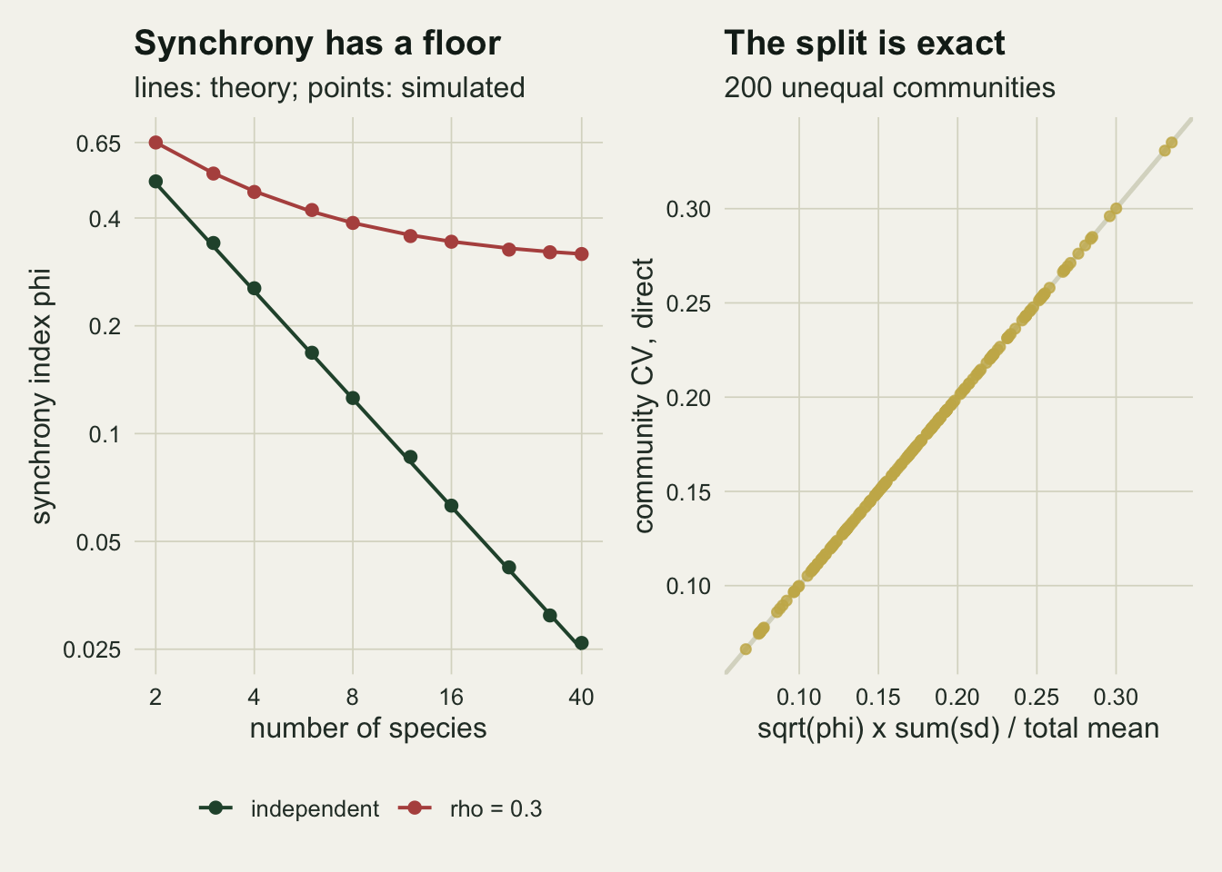
Holding synchrony fixed: the mean-variance route
Now give the community S equal species that share a fixed total mean, so each species has mean mu_T / S and standard deviation c * (mu_T / S)^(z/2). The second factor of the split becomes
sum_i sigma_i / mu_T = S * c * (mu_T / S)^(z/2) / mu_T = c * mu_T^(z/2 - 1) * S^(1 - z/2)
If phi is held at one value while species are added, the only S in the community CV is in that factor, so on log-log axes CV against S is a straight line of slope 1 - z/2. Under these assumptions (equal species, a fixed total, one shared mean-variance law, the correlation adjusted so that phi does not move) this is the entire effect of species number, and it is the same exponent as in the biodiversity post, now applied to the division of a fixed total rather than to a growth in the total. For z below two it is positive: the community gets less stable as species are added, because small populations are proportionally noisier. At z equal to two it is zero, and above two it is negative.
To hold phi fixed, the common correlation for S species is set to rho = (phi * S - 1) / (S - 1), which is negative whenever S is smaller than one over phi and still gives a valid correlation matrix. With phi fixed at 0.25 this needs at least two species, which is why the grid starts at two; one species always has phi equal to one.
phi_fix <- 0.25
z_set   <- c(1, 1.5, 2)
batch_id <- rep(seq_len(n_batch), length.out = n_rep)
set.seed(1998)
fix_runs <- lapply(z_set, function(z) {
  cv_mat <- sapply(S_grid, function(S) {
    rho <- (phi_fix * S - 1) / (S - 1)
    cor_mat <- matrix(rho, S, S); diag(cor_mat) <- 1
    ch <- chol(cor_mat)
    replicate(n_rep, cv_total(sim_comm(rep(mu_tot / S, S), rho, z, n_year, ch)))
  })
  slope_all <- coef(lm(log(colMeans(cv_mat)) ~ log(S_grid)))[2]
  slope_bat <- sapply(seq_len(n_batch), function(b) {
    coef(lm(log(colMeans(cv_mat[batch_id == b, ])) ~ log(S_grid)))[2]
  })
  list(z = z, cv_mean = colMeans(cv_mat), slope = unname(slope_all),
       slope_se = sd(slope_bat) / sqrt(n_batch), theory = 1 - z / 2)
})
fix_tab <- data.frame(z = z_set,
                      slope = sapply(fix_runs, `[[`, "slope"),
                      slope_se = sapply(fix_runs, `[[`, "slope_se"),
                      theory = sapply(fix_runs, `[[`, "theory"))
fix_tab$gap_se <- (fix_tab$slope - fix_tab$theory) / fix_tab$slope_se
fix_pts <- do.call(rbind, lapply(fix_runs, function(r) {
  data.frame(S = S_grid, z = r$z, cv = r$cv_mean,
             cv_line = sqrt(phi_fix) * c_tay * mu_tot^(r$z / 2 - 1) *
                       S_grid^(1 - r$z / 2))
}))
The measured slopes at a synchrony of 0.25 are 0.501 for z of one, 0.249 for z of one and a half, and 0.002 for z of two, against theoretical values of 0.50, 0.25 and 0.00. The batch Monte Carlo standard errors are 0.0016, 0.0029 and 0.0018, and the largest gap is 1.1 standard errors.
ggplot(fix_pts, aes(S, cv, colour = factor(z), linetype = factor(z),
                    shape = factor(z))) +
  geom_line(aes(y = cv_line), linewidth = 0.7) +
  geom_point(size = 2.2) +
  scale_x_log10(breaks = c(2, 4, 8, 16, 40)) +
  scale_y_log10(breaks = c(0.03, 0.05, 0.075, 0.1, 0.15, 0.2),
                labels = function(b) sprintf("%g", b)) +
  scale_colour_manual(values = c(te_gold, te_body, te_ink),
                      labels = c("z = 1", "z = 1.5", "z = 2"), name = NULL) +
  scale_linetype_manual(values = c("solid", "dashed", "dotted"),
                        labels = c("z = 1", "z = 1.5", "z = 2"), name = NULL) +
  scale_shape_manual(values = c(16, 17, 15),
                     labels = c("z = 1", "z = 1.5", "z = 2"), name = NULL) +
  labs(x = "number of species (log scale)", y = "community CV (log scale)",
       title = "At fixed synchrony, the slope is 1 - z/2",
       subtitle = "fixed total mean, equal species, phi = 0.25") +
  theme_datasheet() +
  theme(legend.position = "bottom")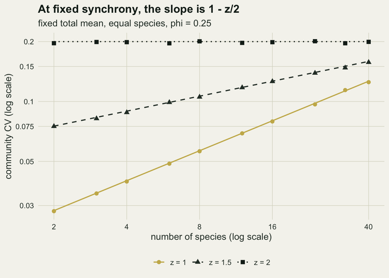
Holding richness fixed: the synchrony route
The other factor is handled the same way. At a fixed number of species and fixed means, the sum of standard deviations does not change, and the community CV is proportional to the square root of phi. The sweep uses sixteen species and synchrony from 0.05 to 0.95.
S_sweep   <- 16
phi_sweep <- seq(0.05, 0.95, by = 0.10)
set.seed(2013)
sweep_cv <- sapply(phi_sweep, function(ph) {
  rho <- (ph * S_sweep - 1) / (S_sweep - 1)
  cor_mat <- matrix(rho, S_sweep, S_sweep); diag(cor_mat) <- 1
  ch <- chol(cor_mat)
  replicate(n_rep, cv_total(sim_comm(rep(mu_tot / S_sweep, S_sweep), rho,
                                     z_main, n_year, ch)))
})
sweep_df <- data.frame(phi = phi_sweep, cv = colMeans(sweep_cv),
                       cv_se = apply(sweep_cv, 2, sd) / sqrt(n_rep))
sum_sd_ratio <- S_sweep * c_tay * (mu_tot / S_sweep)^(z_main / 2) / mu_tot
sweep_df$cv_line <- sqrt(sweep_df$phi) * sum_sd_ratio
sweep_slope <- coef(lm(log(cv) ~ log(phi), data = sweep_df))[2]
sweep_ratio <- sweep_df$cv[nrow(sweep_df)] / sweep_df$cv[1]
sweep_ratio_true <- sqrt(max(phi_sweep) / min(phi_sweep))
sweep_bias <- mean(sweep_df$cv / sweep_df$cv_line)
The log-log slope of mean community CV on phi is 0.501, against one half. Moving from the least to the most synchronous community in the sweep multiplies the CV by 4.34, and the square-root law predicts 4.36. The simulated means sit on average at 0.993 of the line, mainly because the sample standard deviation in a thirty-year series is biased slightly downwards; the bias is a constant factor and does not alter the slope.
sweep_cloud <- data.frame(phi = rep(phi_sweep, each = n_rep),
                          cv = as.vector(sweep_cv))
ggplot(sweep_df, aes(phi, cv)) +
  geom_jitter(data = sweep_cloud, width = 0.012, height = 0,
              colour = te_line, size = 0.6, alpha = 0.6) +
  geom_line(aes(y = cv_line), colour = te_ink, linewidth = 0.8) +
  geom_point(colour = te_gold, size = 2.4) +
  scale_x_continuous(breaks = phi_sweep) +
  labs(x = "synchrony index phi", y = "community CV",
       title = "At fixed richness, CV goes as the square root of phi",
       subtitle = "sixteen species, z = 1.5, thirty-year series") +
  theme_datasheet()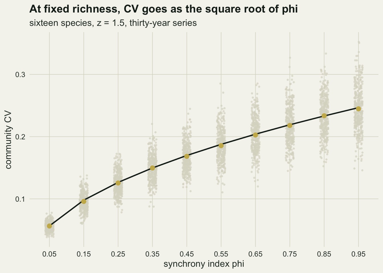
Independence is a synchrony assumption
The classic statistical-averaging argument (Doak et al. 1998; Tilman, Lehman and Bristow 1998) takes species to fluctuate independently, and Tilman (1999) lists the resulting portfolio effect among the general consequences of diversity. In the split, that is not an absence of assumptions about synchrony; it is the specific assumption phi = 1/S. Putting it into the community CV gives
CV_com = c * mu_T^(z/2 - 1) * S^(1 - z/2) * S^(-1/2) = c * mu_T^(z/2 - 1) * S^((1 - z)/2)
so the independent slope (1 - z)/2 is the sum of the mean-variance slope 1 - z/2 and a synchrony slope of minus one half. Independence stabilises the total with added species only when z exceeds one, and at z of one and a half the stabilising synchrony term is twice the size of the destabilising mean-variance term.
The counter-example is a community whose species share a response to the same driver. A pairwise correlation of 0.8 is a strong shared response, chosen to make the contrast plain. The mean-variance exponent is left at 1.5, exactly as in the independent community.
rho_shared <- 0.8
S_full <- c(1, S_grid)
set.seed(1999)
shared_runs <- do.call(rbind, lapply(c(0, rho_shared), function(rho) {
  cv_mat <- sapply(S_full, function(S) {
    cor_mat <- matrix(rho, S, S); diag(cor_mat) <- 1
    ch <- chol(cor_mat)
    replicate(n_rep, cv_total(sim_comm(rep(mu_tot / S, S), rho, z_main,
                                       n_year, ch)))
  })
  slope_bat <- sapply(seq_len(n_batch), function(b) {
    coef(lm(log(colMeans(cv_mat[batch_id == b, ])) ~ log(S_full)))[2]
  })
  data.frame(S = S_full, rho = rho, cv = colMeans(cv_mat),
             cv_line = cv_theory(S_full, rho, z_main),
             slope = unname(coef(lm(log(colMeans(cv_mat)) ~ log(S_full)))[2]),
             slope_se = sd(slope_bat) / sqrt(n_batch))
}))
ind_run <- shared_runs[shared_runs$rho == 0, ]
shr_run <- shared_runs[shared_runs$rho == rho_shared, ]
ind_fold <- ind_run$cv[ind_run$S == 40] / ind_run$cv[ind_run$S == 1]
shr_fold <- shr_run$cv[shr_run$S == 40] / shr_run$cv[shr_run$S == 1]
shr_phi40 <- rho_shared + (1 - rho_shared) / 40
fold_z2 <- cv_theory(40, rho_shared, 2) / cv_theory(1, rho_shared, 2)
With independent species the fitted slope over one to forty species is -0.248 (Monte Carlo standard error 0.0020, theory -0.25), and the community CV at forty species is 0.40 times its single-species value. With the shared response the slope is +0.228 (standard error 0.0020), and forty species give 2.29 times the single-species CV. The total became less stable as species were added. Synchrony at forty species is 0.805, so the synchrony factor fell by only 10 per cent from its single-species value, while the mean-variance factor rose by 151 per cent. The straight-line slope is a summary of a curve here, because phi approaches its floor gradually, which is why it differs from the limiting slope of 0.25.
The same shared response with z equal to two gives a forty-species CV of 0.897 times the single-species value by the formula, and all of that change comes from the synchrony factor, because the mean-variance factor is flat at z of two. In neither version does any species compensate for another, and nothing in the simulation interacts.
ggplot(shared_runs, aes(S, cv, colour = factor(rho))) +
  geom_line(aes(y = cv_line), linewidth = 0.7) +
  geom_point(size = 2.2) +
  scale_x_log10(breaks = c(1, 2, 4, 8, 16, 40)) +
  scale_y_log10(breaks = c(0.05, 0.075, 0.1, 0.15, 0.2, 0.3),
                labels = function(b) sprintf("%g", b)) +
  scale_colour_manual(values = c(te_forest, te_rust),
                      labels = c("independent", "shared response, rho = 0.8"),
                      name = NULL) +
  labs(x = "number of species (log scale)", y = "community CV (log scale)",
       title = "Same exponent, opposite diversity slope",
       subtitle = "z = 1.5, fixed total mean") +
  theme_datasheet() +
  theme(legend.position = "bottom")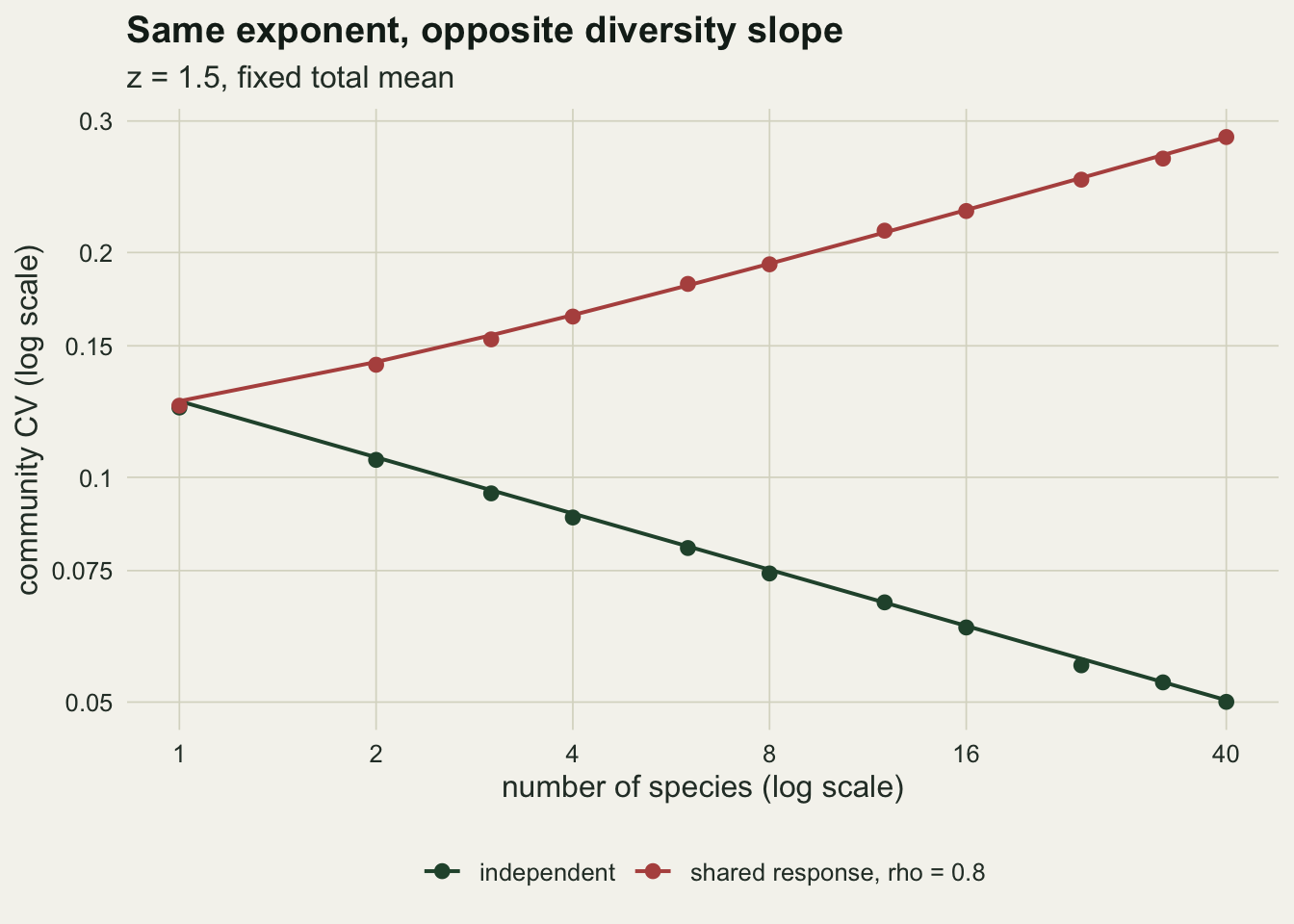
What to report
n_short   <- c(10, 30)
n_rep_sh  <- 10000  # more replicates here: the bias is a few per cent
rho_short <- 0.3
c4 <- function(n) sqrt(2 / (n - 1)) * exp(lgamma(n / 2) - lgamma((n - 1) / 2))
sd_eq  <- c_tay * (mu_tot / S_sweep)^(z_main / 2)
set.seed(4766)
short_runs <- do.call(rbind, lapply(c(0, rho_short), function(rho) {
  cor_mat <- matrix(rho, S_sweep, S_sweep); diag(cor_mat) <- 1
  ch <- chol(cor_mat)
  phi_true <- rho + (1 - rho) / S_sweep
  varT_true <- S_sweep * sd_eq^2 * (1 + (S_sweep - 1) * rho)
  do.call(rbind, lapply(n_short, function(n_yr) {
    draws <- replicate(n_rep_sh, {
      abund <- sim_comm(rep(mu_tot / S_sweep, S_sweep), rho, z_main, n_yr, ch)
      c(sync_phi(abund), var(rowSums(abund)))
    })
    data.frame(rho = rho, n = n_yr, phi_true = phi_true,
               phi_mean = mean(draws[1, ]),
               factor = mean(draws[1, ]) / phi_true,
               factor_se = sd(draws[1, ]) / sqrt(n_rep_sh) / phi_true,
               varT_ratio = mean(draws[2, ]) / varT_true,
               c4_factor = 1 / c4(n_yr)^2)
  }))
}))
sh_i10 <- short_runs[short_runs$rho == 0 & short_runs$n == 10, ]
sh_i30 <- short_runs[short_runs$rho == 0 & short_runs$n == 30, ]
sh_c10 <- short_runs[short_runs$rho == rho_short & short_runs$n == 10, ]
neg_share <- mean(sim_comm(rep(mu_tot / 40, 40), 0, 2, 2000) < 0)
Report phi together with the abundance-weighted mean species CV, not the community CV alone. The community CV is their product (after a square root), and a single number cannot say which factor moved between two treatments. Loreau and de Mazancourt (2008) argue that independence is a weak null and compare observed synchrony with the value from a neutral model, so state which reference value is used. For independent equal species it is one over S, and a measured phi near one over S is not evidence of compensation.
State the length of the series. With sixteen independent species the true phi is 0.0625; over 10000 simulated communities the mean estimate is 0.0637 in thirty-year series and 0.0659 in ten-year series. In ten-year series that is 1.055 times the true value (Monte Carlo standard error 0.005), and in thirty-year series 1.018 (standard error 0.003). The cause is the denominator. The variance of the total is unbiased (its simulated mean is 1.000 times the true value in ten-year series), but the sample standard deviation of each species is biased downwards by the factor c4, which for Gaussian data depends only on the series length, so the squared sum of standard deviations is too small and phi is inflated by roughly one over c4 squared. That factor is 1.057 for ten years and 1.017 for thirty, in line with the simulated factors. It is only a first-order account, because phi is a ratio of two random quantities. When species are positively correlated the numerator and denominator err together and the bias largely cancels: with a pairwise correlation of 0.3 the ten-year factor is 1.004 (standard error 0.003). A ten-year phi for a species-rich, weakly synchronous community is therefore read a few per cent high.
If a diversity-stability slope is reported, report the mean-variance exponent that goes with it. The same slope can come from asynchrony or from the exponent, and the derivation above shows that at fixed synchrony the slope is 1 - z/2, which alone can be positive, zero or negative. The exponent should be fitted on the temporal mean and variance of the species in the same data, since the value from a spatial survey of quadrats need not match it.
Honest limits
The slope derivations assume equal species sharing a fixed total, one mean-variance law for all of them and a single correlation for every pair. Real communities have dominant species, and the weighted mean CV then depends on which species are dominant as much as on how many species there are. The split itself does not need any of these assumptions; the power laws for the slope do.
The total mean is held constant as species are added. In a biodiversity experiment the total usually rises with richness, and that adds the mu^(1 - z/2) gain from the biodiversity post on top of everything here. That gain multiplies the two factors here, so a measured slope from an experiment where the total grows mixes all three.
Abundances are Gaussian. With z equal to two and forty species, 0.60 per cent of simulated abundances in an independent community were negative, and 0.96 per cent of all abundances in the unequal communities of the identity check. The split is unaffected, because it is algebra on whatever numbers are given, but a real biomass series cannot go below zero and its variance near zero is not Gaussian.
Phi describes synchrony and says nothing about its cause. The same value can come from a shared environmental driver, from compensating responses, or from drift, and Loreau and de Mazancourt (2008) show in a neutral model that per capita growth rates can be strongly synchronised while population sizes are desynchronised by ecological drift, so the index depends on which variable is measured. A low phi is a pattern that invites a mechanism, not evidence for one. Pairwise correlations were identical within each simulated community; with a mixture of positive and negative pairs, the same phi can hide very different pair structures.
References
Loreau M, de Mazancourt C 2008 American Naturalist 172(2):E48-E66 (10.1086/589746)
Loreau M, de Mazancourt C 2013 Ecology Letters 16(s1):106-115 (10.1111/ele.12073)
Doak DF, Bigger D, Harding EK, Marvier MA, O’Malley RE, Thomson D 1998 American Naturalist 151(3):264-276 (10.1086/286117)
Tilman D, Lehman CL, Bristow CE 1998 American Naturalist 151(3):277-282 (10.1086/286118)
Tilman D 1999 Ecology 80(5):1455-1474 (10.1890/0012-9658(1999)080[1455:TECOCI]2.0.CO;2)