---
title: "Step lengths and turning angles in R"
description: "Turn an animal track into step lengths and turning angles in R, fit the distributions, and see why path length and tortuosity depend on the fix interval."
date: "2026-07-09 10:00"
categories: [R, MASS, movement ecology, telemetry, ecology tutorial]
image: thumbnail.png
image-alt: "A winding correlated random walk trajectory with a marked start and end point, drawn in forest green on a pale background."
---
A movement track is a sequence of relocations in time. The two quantities that describe how an animal moves between them are the step length (distance from one fix to the next) and the turning angle (the change in direction at each fix). Together they define a random-walk model of the path, and they feed directly into step selection functions. This post extracts both from a synthetic track using base R plus `MASS`, fits the step-length distribution, summarises the turning angles with circular statistics, and then shows the catch that trips up every movement study: both descriptors depend on how often you sampled, not on the animal alone.
## A correlated random walk
We simulate a correlated random walk (CRW): step lengths drawn from a gamma distribution and turning angles from a wrapped normal centred on zero, so the animal tends to keep going in roughly the same direction. Cumulating the steps gives the track. Coordinates are in metres and the data are illustrative.
```{r}
#| label: setup
#| include: false
te_ink <- "#16241d"; te_body <- "#2c3a31"; te_forest <- "#275139"
te_label <- "#46604a"; te_sage <- "#93a87f"; te_paper <- "#f5f4ee"
te_line <- "#dad9ca"; te_faint <- "#5d6b61"; te_gold <- "#cda23f"; te_red <- "#b5534e"
theme_te <- function(base_size = 12) {
ggplot2::theme_minimal(base_size = base_size) +
ggplot2::theme(
text = ggplot2::element_text(colour = te_body),
plot.title = ggplot2::element_text(colour = te_ink, face = "bold"),
plot.subtitle = ggplot2::element_text(colour = te_faint),
axis.title = ggplot2::element_text(colour = te_label),
axis.text = ggplot2::element_text(colour = te_faint),
panel.grid.major = ggplot2::element_line(colour = te_line, linewidth = 0.3),
panel.grid.minor = ggplot2::element_blank(),
plot.background = ggplot2::element_rect(fill = te_paper, colour = NA),
panel.background = ggplot2::element_rect(fill = te_paper, colour = NA),
legend.key = ggplot2::element_blank(),
legend.title = ggplot2::element_text(colour = te_label),
strip.text = ggplot2::element_text(colour = te_ink, face = "bold"))
}
```
```{r}
#| label: data
#| message: false
library(MASS); library(ggplot2); library(dplyr)

set.seed(5122)
n <- 500
sl <- rgamma(n, shape = 2, scale = 15)   # step lengths (m)
turn <- rnorm(n, 0, 0.8)                  # turning angles, wrapped normal
head <- cumsum(turn)                      # absolute heading
pos <- data.frame(x = c(0, cumsum(sl * cos(head))),
                  y = c(0, cumsum(sl * sin(head))))
round(c(steps = n, extent_x = diff(range(pos$x)), extent_y = diff(range(pos$y))))
```
The track has 500 steps and spans roughly 1.5 by 2.3 km. From the coordinates alone we recover the step lengths and turning angles, which is what you would do with real GPS data: the generating values are not observed, only the positions.
```{r}
#| label: extract
step <- sqrt(diff(pos$x)^2 + diff(pos$y)^2)              # step lengths
bear <- atan2(diff(pos$y), diff(pos$x))                 # bearing of each step
tn <- diff(bear); tn <- (tn + pi) %% (2 * pi) - pi      # turning angle, wrapped to (-pi, pi]
round(c(mean_step = mean(step), median_step = median(step), max_step = max(step)), 1)
```
## Fitting the step-length distribution
Step lengths are positive and usually right-skewed with few very short steps, so the exponential (which has its mode at zero) tends to fit poorly. The gamma and Weibull allow a mode away from zero. `MASS::fitdistr` gives maximum-likelihood fits and we compare them by AIC.
```{r}
#| label: fit
#| warning: false
aic <- function(fit, k) -2 * fit$loglik + 2 * k
fe <- fitdistr(step, "exponential")
fg <- fitdistr(step, "gamma")
fw <- fitdistr(step, "weibull")
tab <- data.frame(dist = c("exponential", "gamma", "weibull"),
                  AIC = round(c(aic(fe, 1), aic(fg, 2), aic(fw, 2)), 1))
tab$dAIC <- tab$AIC - min(tab$AIC)
tab
round(c(gamma_shape = fg$estimate[["shape"]],
        gamma_mean = fg$estimate[["shape"]] / fg$estimate[["rate"]]), 2)
```
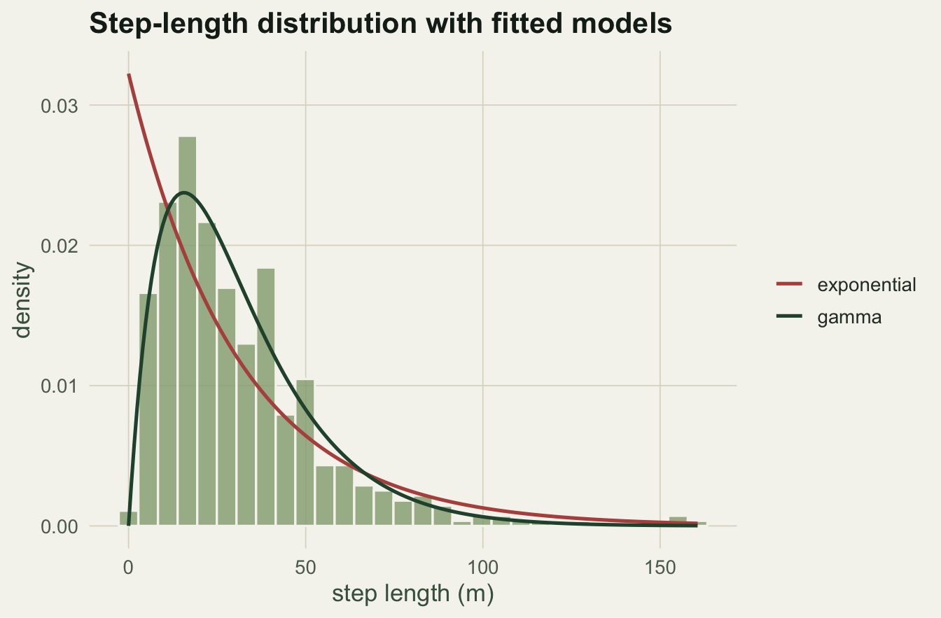
The gamma wins, with an AIC 117 units below the exponential and 18 below the Weibull. Its shape parameter is 2.02 and the mean step is 31 m, close to the values used to generate the track. The exponential misses because it forces the most likely step length to be zero, while the data have a clear mode around 15 to 20 m.
```{r}
#| label: fig-steplength
#| fig-cap: "Step-length histogram with maximum-likelihood exponential and gamma fits. The gamma captures the mode near 15 to 20 m; the exponential is monotone and cannot."
#| fig-alt: "A right-skewed histogram of step lengths with a green gamma curve peaking near 15 to 20 metres and a red exponential curve that only decreases from zero."
#| fig-width: 7
#| fig-height: 4.6
xs <- seq(0, max(step), length.out = 200)
dens <- rbind(
  data.frame(x = xs, d = dexp(xs, rate = fe$estimate["rate"]), fit = "exponential"),
  data.frame(x = xs, d = dgamma(xs, shape = fg$estimate["shape"], rate = fg$estimate["rate"]), fit = "gamma"))
ggplot() +
  geom_histogram(data = data.frame(step = step), aes(step, after_stat(density)),
                 bins = 30, fill = te_sage, colour = te_paper, alpha = 0.8) +
  geom_line(data = dens, aes(x, d, colour = fit), linewidth = 0.9) +
  scale_colour_manual(values = c(exponential = te_red, gamma = te_forest), name = NULL) +
  labs(title = "Step-length distribution with fitted models",
       x = "step length (m)", y = "density") +
  theme_te(13)
```
## Turning angles need circular statistics
Angles wrap around, so the ordinary mean and standard deviation do not apply: the average of 350 and 10 degrees is 0, not 180. The tool is the mean resultant vector. Represent each turn as a unit vector, average the vectors, and the length of that average (the mean resultant length, written R bar) measures concentration: near 1 means the turns cluster tightly around one direction, near 0 means they are spread around the circle. The Rayleigh test asks whether the turns are uniform.
```{r}
#| label: turning
Rbar <- sqrt(mean(cos(tn))^2 + mean(sin(tn))^2)
mang <- atan2(mean(sin(tn)), mean(cos(tn)))
nt <- length(tn); Z <- nt * Rbar^2
p_ray <- exp(-Z) * (1 + (2 * Z - Z^2) / (4 * nt) -
         (24 * Z - 132 * Z^2 + 76 * Z^3 - 9 * Z^4) / (288 * nt^2))
a_inv <- function(R) {
  if (R < 0.53) 2 * R + R^3 + 5 * R^5 / 6
  else if (R < 0.85) -0.4 + 1.39 * R + 0.43 / (1 - R)
  else 1 / (R^3 - 4 * R^2 + 3 * R)
}
round(c(Rbar = Rbar, mean_angle = mang, rayleigh_p = p_ray, kappa = a_inv(Rbar)), 3)
```
The mean resultant length is 0.72 and the mean turn is essentially zero, so the animal turns little on average and holds its heading: this is the directional persistence that makes the walk correlated rather than pure diffusion. The Rayleigh test rejects uniformity overwhelmingly. Converting R bar to a von Mises concentration gives a kappa of 2.13, which is the parameter a step selection or state-space model would carry.
## The metrics depend on the fix interval
Here is the part that matters for interpretation. A track sampled less often cuts the corners of the real path, so it looks straighter and shorter. We thin the track by keeping every m-th fix and recompute the total path length and the turning concentration at each interval.
```{r}
#| label: scaling
thin_metrics <- function(pos, m) {
  p <- pos[seq(1, nrow(pos), by = m), ]
  s <- sqrt(diff(p$x)^2 + diff(p$y)^2)
  b <- atan2(diff(p$y), diff(p$x)); t <- diff(b); t <- (t + pi) %% (2 * pi) - pi
  data.frame(m = m, path = sum(s), mean_step = mean(s),
             Rbar = sqrt(mean(cos(t))^2 + mean(sin(t))^2))
}
sc <- do.call(rbind, lapply(c(1, 2, 3, 4, 6, 8), thin_metrics, pos = pos))
sc$path_rel <- sc$path / sc$path[1]; sc$Rbar_rel <- sc$Rbar / sc$Rbar[1]
round(sc, 3)
```
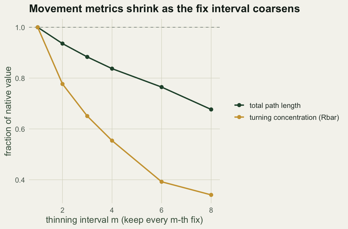
At the native resolution the path is 15.5 km long with a turning concentration of 0.72. Keep only every eighth fix and the measured path falls to 10.5 km, a 32% underestimate, while the concentration drops to 0.25: the same movement now looks far more diffuse. The mean step grows from 31 to 169 m simply because each retained step spans a longer gap. None of this reflects a change in behaviour; it is the sampling interval. The effect is stronger for more tortuous paths and has been quantified for real tracking data (Rowcliffe 2012).
```{r}
#| label: fig-scaling
#| fig-cap: "Total path length and turning concentration relative to the native fix rate, as the track is thinned. Both shrink as the interval coarsens."
#| fig-alt: "Two lines against thinning interval: path length falls gently to about 0.68 of its full value and turning concentration falls steeply to about 0.34, both below a dashed reference line at one."
#| fig-width: 7
#| fig-height: 4.6
scl <- rbind(
  data.frame(m = sc$m, value = sc$path_rel, metric = "total path length"),
  data.frame(m = sc$m, value = sc$Rbar_rel, metric = "turning concentration (Rbar)"))
ggplot(scl, aes(m, value, colour = metric)) +
  geom_hline(yintercept = 1, linetype = "dashed", colour = te_faint, linewidth = 0.3) +
  geom_line(linewidth = 0.9) + geom_point(size = 2) +
  scale_colour_manual(values = c("total path length" = te_forest,
                                 "turning concentration (Rbar)" = te_gold), name = NULL) +
  labs(title = "Movement metrics shrink as the fix interval coarsens",
       x = "thinning interval m (keep every m-th fix)", y = "fraction of native value") +
  theme_te(13)
```
## What to take away
Step lengths and turning angles are the raw material of movement analysis, but they are properties of the observation scale as much as the animal. Fit the step-length distribution rather than assuming exponential; the mode away from zero usually favours a gamma or Weibull. Summarise turning angles with the resultant vector, never the arithmetic mean. Above all, report the fix interval and treat path length and tortuosity as scale-dependent: a distance travelled or a straightness index means nothing without the sampling rate attached, and two studies on different schedules are not comparable. The step-and-angle pair is also the basis of the correlated random walk and step selection models, which the next posts build on.
## References
Kareiva & Shigesada 1983 Oecologia 56(2-3):234-238 (10.1007/BF00379695)
Turchin 1998 Quantitative Analysis of Movement, Sinauer Associates, ISBN 978-0-87893-847-8
Codling, Plank & Benhamou 2008 Journal of the Royal Society Interface 5(25):813-834 (10.1098/rsif.2008.0014)
Rowcliffe, Carbone, Kays, Kranstauber & Jansen 2012 Methods in Ecology and Evolution 3(4):653-662 (10.1111/j.2041-210X.2012.00197.x)
Batschelet 1981 Circular Statistics in Biology, Academic Press, ISBN 978-0-12-081050-9
## Related tutorials
- [Home ranges: MCP versus kernel density](../home-range-mcp-kde/)
- [Correlated random walks and net displacement](../correlated-random-walk/)
- [Resource selection functions](../resource-selection-functions/)
- [Kaplan-Meier survival curves](../kaplan-meier-survival-curves/)