library(ggplot2)
library(patchwork)

te_paper  <- "#f5f4ee"
te_ink    <- "#16241d"
te_body   <- "#2c3a31"
te_forest <- "#275139"
te_rust   <- "#b5534e"
te_gold   <- "#c9b458"
te_line   <- "#dad9ca"

theme_datasheet <- function() {
  theme_minimal(base_size = 12) +
    theme(plot.background  = element_rect(fill = te_paper, colour = NA),
          panel.background = element_rect(fill = te_paper, colour = NA),
          panel.grid.major = element_line(colour = te_line, linewidth = 0.3),
          panel.grid.minor = element_blank(),
          text             = element_text(colour = te_body),
          plot.title       = element_text(colour = te_ink, face = "bold"),
          plot.subtitle    = element_text(colour = te_body),
          axis.text        = element_text(colour = te_body))
}Standardising variables before clustering sites
R
clustering
multivariate
standardisation
simulation
ecology tutorial
Z-scores, range or MAD before k-means? Simulated site typologies in R show the shape of the variables carrying no groups decides which scaler works best.
A wetland survey has eighty sites and a vegetation typology that the field team trusts: forty poor fens, twenty-five rich fens and fifteen transitional mires. The question for the analysis is whether the environmental measurements recover that typology on their own, so that new sites can be placed without a botanist. Six variables were measured at every site, in six different units. Two of them, say pH and calcium, carry the difference between the types. The other four carry none: the altitude of each site on a transect laid out at even steps, the water depth at the sampling point, and two nutrient concentrations that vary from site to site for reasons unrelated to fen type. Nobody knows in advance which variables are which, so all six go into k-means, and before that every analyst standardises.
Standardising is not the contested step; the choice of divisor is. The three candidates in common use are the z-score, which subtracts the mean and divides by the standard deviation (scale() in base R), range scaling, which maps every variable onto zero to one (decostand(x, method = "range") in vegan), and an outlier-resistant version that subtracts the median and divides by the median absolute deviation. Milligan and Cooper compared standardisations in a large simulation study in 1988 and found that dividing by the range recovered the planted clusters best, and Steinley and Brusco later built a variable weighting procedure for k-means on the ratio of a variable’s variance to its range, the quantity that explains why. This post is a demonstration of that published result first, and then of its limit. What is measured here, and not taken from the literature, is how the ranking behaves when the variables with no groups in them are flat gradients rather than bell-shaped noise, what one extreme site does to it, whether the usual log transformation changes the answer, and whether a one-line check of each variable picks the right scaler.
The site already covers the step before this one. PCA for environmental data shows that raw units must not be left alone: unscaled, the variable measured in the largest numbers takes the first axis. Its only comparison is raw against z-scored. The question it leaves is which normaliser, and the answer turns on the shape of the variables that carry no groups at all. The hierarchical clustering post works on species counts through Bray-Curtis dissimilarity, where no scaling question arises. Checking a functional diversity analysis builds its trait distance as Gower’s coefficient, which divides every continuous trait by its range, so range scaling is already the default there without being examined. The same family of problem, a normaliser that silently sets the weights, appears in a decision table in structured decision making, where three rescalings of four objectives are compared. The natural next step after this post is checking a community classification, which asks whether a typology produced by a clustering is more than noise.
Eighty sites, three types, six variables
The simulation keeps the survey’s structure and nothing else. Eighty sites fall into three types of 40, 25 and 15. The two informative variables place the three type centres on a triangle whose side is d within-type standard deviations, so d is the separation of the types in the only variables that know about them. The four uninformative variables take one of four shapes: bell-shaped normal noise, a flat gradient (sites spread evenly along a designed transect, which gives a uniform distribution), right-skewed lognormal noise of the kind raw nutrient concentrations show, or two flat gradients plus two skewed variables. Every column is then multiplied by its own arbitrary unit factor, between exp(-3) and exp(3), so that clustering the raw values would be meaningless and some standardisation is compulsory.
Agreement between the k-means partition and the true types is measured by the adjusted Rand index of Hubert and Arabie: one for perfect recovery, zero for the agreement expected from random labels. It is coded by hand below from its definition, a pair-counting index corrected for chance under fixed marginal totals. Alongside the three scalers, two references ride along in every data set. The first is an oracle that clusters the two informative variables alone, z-scored, which is the ceiling any choice of divisor could reach if the empty variables were simply dropped. The second is a weighting in the spirit of Steinley and Brusco: range-scale, then weight each variable by the square root of its share of the total variance-to-range ratio. That is a simplified version for comparison, not their published procedure, which adds a variable selection step.
adj_rand <- function(a, b) {
  tab <- table(a, b)
  n_obs  <- sum(tab)
  s_cell <- sum(choose(tab, 2))
  s_row  <- sum(choose(rowSums(tab), 2))
  s_col  <- sum(choose(colSums(tab), 2))
  expect <- s_row * s_col / choose(n_obs, 2)
  (s_cell - expect) / ((s_row + s_col) / 2 - expect)
}
scale_z     <- function(x) scale(x)
scale_range <- function(x) apply(x, 2, function(v) (v - min(v)) / diff(range(v)))
scale_mad   <- function(x) apply(x, 2, function(v) (v - median(v)) / mad(v))
range_sd    <- function(x) apply(x, 2, function(v) diff(range(v)) / sd(v))
rule_cut    <- 3.7

make_sites <- function(d_sep, shape, n_noise = 4, sizes = c(40, 25, 15),
                       outlier = FALSE, log_what = "none") {
  type_id <- rep(1:3, sizes)
  n_site  <- length(type_id)
  centres <- cbind(c(0, d_sep, d_sep / 2), c(0, 0, d_sep * sqrt(3) / 2))
  informative <- centres[type_id, ] + matrix(rnorm(n_site * 2), n_site, 2)
  noise <- switch(shape,
    normal    = matrix(rnorm(n_site * n_noise), n_site),
    uniform   = matrix(runif(n_site * n_noise), n_site),
    lognormal = matrix(rlnorm(n_site * n_noise, 0, 0.8), n_site),
    mixed     = cbind(matrix(runif(n_site * 2), n_site),
                      matrix(rlnorm(n_site * 2, 0, 0.8), n_site)))
  if (log_what == "skewed") noise[, 3:4] <- log(noise[, 3:4])
  if (log_what == "all") noise <- log(noise)
  x_raw <- cbind(informative, noise)
  if (outlier) x_raw[1, 1] <- x_raw[1, 1] + 8
  x_raw <- sweep(x_raw, 2, exp(runif(ncol(x_raw), -3, 3)), "*")
  list(x = x_raw, type_id = type_id)
}

cluster_set <- function(d_sep, shape, ward = FALSE, ...) {
  s <- make_sites(d_sep, shape, ...)
  scaled <- list(z = scale_z(s$x), range = scale_range(s$x), mad = scale_mad(s$x))
  vr <- apply(scaled$range, 2, var)
  scaled$vr_weight <- sweep(scaled$range, 2, sqrt(vr / sum(vr)), "*")
  scaled$oracle <- scale_z(s$x[, 1:2])
  km <- vapply(scaled, function(xs)
    adj_rand(kmeans(xs, 3, nstart = 20, iter.max = 50)$cluster, s$type_id), 0)
  pick_z <- any(range_sd(s$x) < rule_cut)
  out <- c(km, rule = if (pick_z) km[["z"]] else km[["range"]], pick_z = pick_z)
  if (ward) {
    wd <- vapply(scaled[c("z", "range", "mad")], function(xs)
      adj_rand(cutree(hclust(dist(xs), "ward.D2"), 3), s$type_id), 0)
    out <- c(out, ward_z = wd[["z"]], ward_range = wd[["range"]], ward_mad = wd[["mad"]])
  }
  out
}
The rule entry and the rule_cut constant belong to the check described in the last results section; they are computed here so that the check is scored on exactly the data sets the scalers are scored on. The cut of 3.7 was fixed before the grid ran, halfway between the flat value and the informative value that a pilot run gave for this geometry (the ratio section below measures both again); the limits section says what happens when the groups sit further apart.
Before the full grid, one data set shows what the index is measuring. This is the hardest shape mix, two flat gradients and two skewed variables, at a type separation of four standard deviations, clustered three times.
set.seed(2029)
ex <- make_sites(4, "mixed")
ex_scaled <- list(`z-score` = scale_z(ex$x), range = scale_range(ex$x),
                  `median and MAD` = scale_mad(ex$x))
ex_part <- lapply(ex_scaled, function(xs) kmeans(xs, 3, nstart = 20, iter.max = 50)$cluster)
ex_ari  <- vapply(ex_part, adj_rand, 0, b = ex$type_id)

perms <- rbind(c(1, 2, 3), c(1, 3, 2), c(2, 1, 3), c(2, 3, 1), c(3, 1, 2), c(3, 2, 1))
relabel <- function(cl, truth) {
  hits <- apply(perms, 1, function(p) sum(p[cl] == truth))
  perms[which.max(hits), ][cl]
}
ex_match <- vapply(ex_part, function(cl) mean(relabel(cl, ex$type_id) == ex$type_id), 0)
The three partitions score 0.169 for the z-score, 0.063 for range scaling and -0.013 for the median and MAD. After matching cluster labels to types, the share of sites placed in their own type is 0.62, 0.50 and 0.40. A share can look respectable while the index is low, because with types of 40, 25 and 15 a partition that lumps most sites into one large cluster already places half of them correctly; the adjusted index removes that free agreement.
ex_info <- scale_z(ex$x[, 1:2])
type_names <- c("poor fen", "rich fen", "transitional")
ex_long <- do.call(rbind, lapply(names(ex_part), function(nm) data.frame(
  v1 = ex_info[, 1], v2 = ex_info[, 2],
  true_type = type_names[ex$type_id],
  cluster = type_names[relabel(ex_part[[nm]], ex$type_id)],
  scaler = sprintf("%s: ARI %.2f", nm, ex_ari[[nm]]))))
ex_long$scaler <- factor(ex_long$scaler, levels = unique(ex_long$scaler))

ggplot(ex_long, aes(v1, v2, colour = cluster, shape = true_type)) +
  geom_point(size = 2, stroke = 0.8) +
  facet_wrap(~scaler) +
  scale_colour_manual(values = c(te_forest, te_rust, te_gold), name = "k-means cluster") +
  scale_shape_manual(values = c(16, 17, 1), name = "true type") +
  labs(x = "informative variable 1 (z-score)", y = "informative variable 2 (z-score)",
       title = "The same eighty sites, three typologies") +
  theme_datasheet() +
  theme(legend.position = "bottom", legend.box = "vertical",
        strip.text = element_text(colour = te_ink, face = "bold"))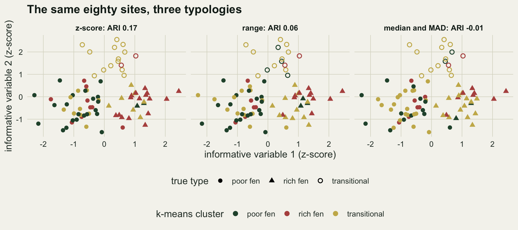
Range scaling wins until the empty variables are flat
The grid crosses type separation (d of 3 and 4) with the four shapes of the uninformative variables and with the presence or absence of one extreme site, which gives sixteen cells. Six extra cells at d of 4, from four extra arms, follow in a later section. Each cell holds five independent draws of sixty data sets. The unit of analysis is the index of one data set of eighty sites; a draw’s value is the mean over its sixty data sets, and the text and figures report the median over the five draws with the lowest and highest draw as the range. A difference such as range minus z is the median of the per-draw differences, so it need not equal the difference of the two medians. k-means runs with twenty random starts in every cell; Ward’s hierarchical method (ward.D2) runs as a check in the cells at d of 4.
cells <- rbind(
  expand.grid(d_sep = c(3, 4), shape = c("normal", "uniform", "lognormal", "mixed"),
              outlier = c(FALSE, TRUE), arm = "grid", n_noise = 4, balanced = FALSE,
              log_what = "none", stringsAsFactors = FALSE),
  data.frame(d_sep = 4, shape = c("normal", "uniform", "normal", "uniform", "mixed", "mixed"),
             outlier = FALSE,
             arm = c("balanced", "balanced", "one variable", "one variable",
                     "log skewed only", "log all four"),
             n_noise = c(4, 4, 1, 1, 4, 4),
             balanced = c(TRUE, TRUE, FALSE, FALSE, FALSE, FALSE),
             log_what = c("none", "none", "none", "none", "skewed", "all")))
n_draw     <- 5
n_per_draw <- 60
n_cells    <- nrow(cells)
n_sets_all <- n_cells * n_draw * n_per_draw

set.seed(4417)
per_set <- vector("list", n_cells)
for (i in seq_len(n_cells)) {
  cl <- cells[i, ]
  sz <- if (cl$balanced) c(27, 27, 26) else c(40, 25, 15)
  m_out <- replicate(n_draw * n_per_draw,
    cluster_set(cl$d_sep, cl$shape, ward = cl$d_sep == 4, n_noise = cl$n_noise,
                sizes = sz, outlier = cl$outlier, log_what = cl$log_what))
  per_set[[i]] <- data.frame(cell = i, draw = rep(seq_len(n_draw), each = n_per_draw),
                             t(m_out))
}

keep_cols <- c("cell", "draw", "z", "range", "mad", "vr_weight", "oracle", "rule", "pick_z")
all_sets  <- do.call(rbind, lapply(per_set, function(p) p[, keep_cols]))
draw_means <- aggregate(cbind(z, range, mad, vr_weight, oracle, rule, pick_z) ~ cell + draw,
                        all_sets, mean)
draw_means$r_minus_z <- draw_means$range - draw_means$z
draw_means$m_minus_z <- draw_means$mad - draw_means$z
cell_med <- aggregate(. ~ cell, draw_means[, names(draw_means) != "draw"], median)
cell_lo  <- aggregate(cbind(z, range, mad, r_minus_z, m_minus_z) ~ cell, draw_means, min)
cell_hi  <- aggregate(cbind(z, range, mad, r_minus_z, m_minus_z) ~ cell, draw_means, max)

cell_of <- function(d, sh, out = FALSE, arm_name = "grid")
  which(cells$d_sep == d & cells$shape == sh & cells$outlier == out & cells$arm == arm_name)
med <- function(i, col) cell_med[[col]][i]
lo  <- function(i, col) cell_lo[[col]][i]
hi  <- function(i, col) cell_hi[[col]][i]

c4n <- cell_of(4, "normal");  c3n <- cell_of(3, "normal")
c4l <- cell_of(4, "lognormal"); c3l <- cell_of(3, "lognormal")
c4u <- cell_of(4, "uniform"); c3u <- cell_of(3, "uniform")
c4m <- cell_of(4, "mixed");   c3m <- cell_of(3, "mixed")
The simulation ran 6600 data sets in total. Under bell-shaped noise at a separation of four, Milligan and Cooper’s result appears as they reported it. k-means after range scaling recovers the types with an index of 0.681, against 0.451 after z-scores and 0.294 after the median and MAD. The gain of range over z is +0.222, and it is not a draw artefact: across the five draws it runs from +0.184 to +0.238. Skewed noise makes range scaling look even better, at 0.712 against 0.468, while the MAD collapses to 0.036, close to the zero of random labels. At a separation of three every index is lower and the ordering holds: 0.340 against 0.234 under normal noise.
Now replace the noise with flat gradients. At a separation of four the range-scaled clustering drops to 0.057, which is almost nothing, while the z-score reaches 0.343 and the MAD 0.584, the best of the three in this cell. Range minus z is now -0.286, from -0.294 to -0.259 over draws. The scaler that won under bell-shaped noise loses here by more than it gained there, on data sets whose informative variables are identical in distribution.
The mixed cell, two flat gradients and two skewed variables, is the one that matters most in practice, because a real survey rarely has four uninformative variables of one shape. There range scaling scores 0.111, the MAD 0.111 and the z-score 0.366. Each of the other two scalers is defeated by one of the two shapes: the range by the flat gradients, the MAD by the skewed variables. The z-score is the only one of the three that stays well clear of zero, although at a level well below the oracle’s 0.862, which is what the same k-means achieves once the four empty variables are left out.
shape_lab <- c(normal = "normal noise", lognormal = "skewed noise",
               uniform = "flat gradients", mixed = "2 flat + 2 skewed")
main_ids <- which(cells$arm == "grid" & !cells$outlier)
main_df <- do.call(rbind, lapply(c("z", "range", "mad"), function(sc) data.frame(
  d_lab  = sprintf("type separation d = %d", cells$d_sep[main_ids]),
  shape  = factor(shape_lab[cells$shape[main_ids]], levels = shape_lab),
  scaler = c(z = "z-score", range = "range", mad = "median and MAD")[[sc]],
  ari = med(main_ids, sc), lo_ari = lo(main_ids, sc), hi_ari = hi(main_ids, sc))))
main_df$scaler <- factor(main_df$scaler, levels = c("z-score", "range", "median and MAD"))
oracle_df <- data.frame(d_lab = sprintf("type separation d = %d", c(3, 4)),
                        oracle = tapply(cell_med$oracle[main_ids], cells$d_sep[main_ids], mean))

ggplot(main_df, aes(shape, ari, colour = scaler)) +
  geom_hline(data = oracle_df, aes(yintercept = oracle), linetype = "dashed",
             colour = te_body, linewidth = 0.5) +
  geom_errorbar(aes(ymin = lo_ari, ymax = hi_ari), width = 0.2, linewidth = 0.5,
                position = position_dodge(width = 0.55)) +
  geom_point(size = 2.6, position = position_dodge(width = 0.55)) +
  facet_wrap(~d_lab) +
  scale_colour_manual(values = c(te_forest, te_gold, te_rust), name = NULL) +
  scale_y_continuous(limits = c(0, 1)) +
  labs(x = "shape of the four variables that carry no types",
       y = "adjusted Rand index to the true types",
       title = "Which scaler wins depends on the empty variables",
       subtitle = "dashed: k-means on the two informative variables alone") +
  theme_datasheet() +
  theme(legend.position = "bottom",
        axis.text.x = element_text(angle = 15, hjust = 1),
        strip.text = element_text(colour = te_ink, face = "bold"))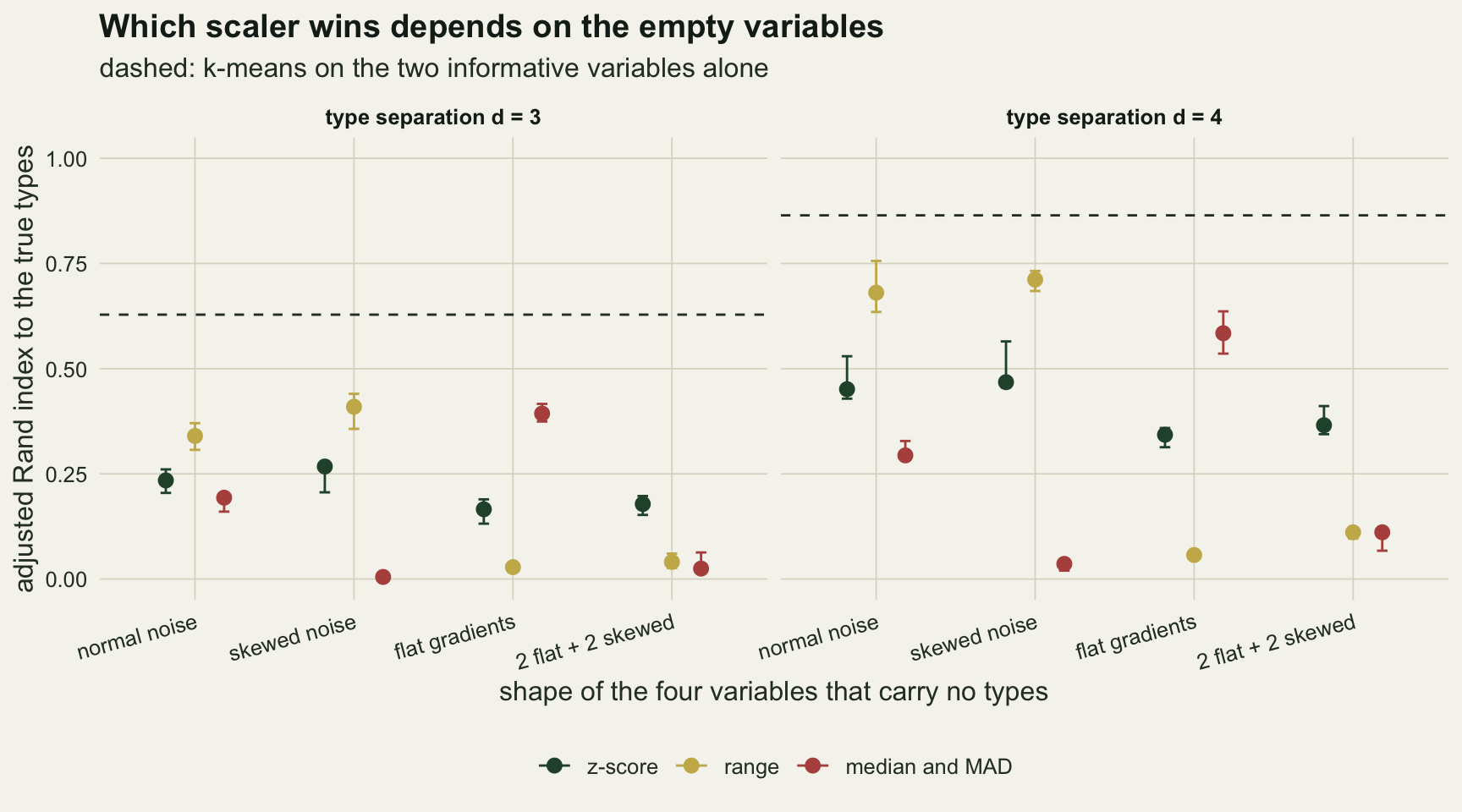
Every divisor is a weight
The explanation is arithmetic, and it is the reason the ranking above is not a surprise once it is written down. k-means on Euclidean distance gives each variable a weight equal to its variance after scaling. A z-score gives every variable a variance of one. Range scaling gives variable j a variance of one over the square of its range-to-SD ratio, and the median and MAD give it the square of its SD-to-MAD ratio. Both ratios are properties of the variable’s shape, and a variable that carries groups has a shape of its own.
n_ratio <- 2000
n_site  <- 80
g_sizes <- rep(1:3, c(40, 25, 15))
ratio_pair <- function(gen) {
  v_mat <- replicate(n_ratio, {
    v <- gen()
    c(range_sd = diff(range(v)) / sd(v), sd_mad = sd(v) / mad(v))
  })
  rowMeans(v_mat)
}
set.seed(7303)
kinds <- list(
  "types, axis 1, d = 4" = function() c(0, 4, 2)[g_sizes] + rnorm(n_site),
  "types, axis 2, d = 4" = function() c(0, 0, 2 * sqrt(3))[g_sizes] + rnorm(n_site),
  "types, axis 1, d = 6" = function() c(0, 6, 3)[g_sizes] + rnorm(n_site),
  "normal noise"         = function() rnorm(n_site),
  "flat gradient"        = function() runif(n_site),
  "skewed noise"         = function() rlnorm(n_site, 0, 0.8),
  "log of a flat gradient" = function() log(runif(n_site)))
ratio_tab <- t(vapply(kinds, ratio_pair, numeric(2)))

unif_closed <- sqrt(12) * (n_site - 1) / (n_site + 1)
unif_mad_closed <- (1 / sqrt(12)) / (qnorm(0.75)^-1 * 0.25)
w_range <- (ratio_tab["types, axis 1, d = 4", "range_sd"] / ratio_tab[, "range_sd"])^2
rs <- function(k) ratio_tab[k, "range_sd"]
sm <- function(k) ratio_tab[k, "sd_mad"]
Averaged over 2000 samples of 80 sites, the range-to-SD ratio is 3.98 for the first informative variable at a separation of four, 4.87 for normal noise, 5.60 for skewed noise and 3.39 for a flat gradient. The flat value has a closed form: the expected range of 80 uniform values is (n - 1)/(n + 1) of the interval, and the standard deviation is the interval over the square root of 12, which gives 3.38.
The second informative variable, on which the fifteen transitional sites sit apart from the other two types, has 4.49, still below both kinds of noise. So range scaling hands a variable with groups in it more variance than normal or skewed noise, because a mixture of separated groups has shorter tails relative to its spread than a single bell does. That is Milligan and Cooper’s result, and it is the observation Steinley and Brusco turned into a weighting. But a flat gradient has even shorter tails than a three-group mixture at this separation: it has none at all. Range scaling therefore gives each flat gradient 1.38 times the variance of the first informative variable, while normal noise gets 0.67 times and skewed noise 0.51 times. The median and MAD reward a different shape: a narrow bulk with a few values far out. A flat gradient has the lowest SD-to-MAD ratio of all, 0.80 (closed form 0.78), below both informative variables (0.87 and 1.28), which is why the MAD did best of the three in the cells whose four empty variables are all flat gradients. Normal noise sits at 1.02, between the two informative variables. Skewed noise sits at 1.72, and because the weight is the square of the ratio, skewed variables outweigh everything else.
These ratios are simple properties of each shape, the flat one in closed form, and they are not the finding. They say which way each scaler pushes; they do not say whether the push is large enough to wreck the partition, and the grid above is what measured that. They also carry a warning for the check in the next section. Groups that sit further apart pull the ratio of an informative variable down: at a separation of six it is 3.56, heading towards the flat value.
ratio_df <- rbind(
  data.frame(kind = rownames(ratio_tab), value = ratio_tab[, "range_sd"],
             measure = "range / SD (range scaling divides by this)"),
  data.frame(kind = rownames(ratio_tab), value = ratio_tab[, "sd_mad"],
             measure = "SD / MAD (MAD scaling multiplies by this)"))
ratio_df$kind <- factor(ratio_df$kind, levels = rev(rownames(ratio_tab)))
ratio_df$measure <- factor(ratio_df$measure, levels = unique(ratio_df$measure))
ratio_df$group <- ifelse(grepl("^types", ratio_df$kind), "carries the types", "carries none")
cut_df <- data.frame(measure = factor("range / SD (range scaling divides by this)",
                                      levels = levels(ratio_df$measure)), cut = rule_cut)

ggplot(ratio_df, aes(value, kind, colour = group)) +
  geom_vline(data = cut_df, aes(xintercept = cut), linetype = "dashed",
             colour = te_rust, linewidth = 0.6) +
  geom_point(size = 3) +
  facet_wrap(~measure, scales = "free_x") +
  scale_colour_manual(values = c(te_forest, te_gold), name = NULL) +
  labs(x = NULL, y = NULL, title = "Each divisor rewards a different shape",
       subtitle = "dashed red: the cut used by the check below") +
  theme_datasheet() +
  theme(legend.position = "bottom", strip.text = element_text(colour = te_ink, face = "bold"))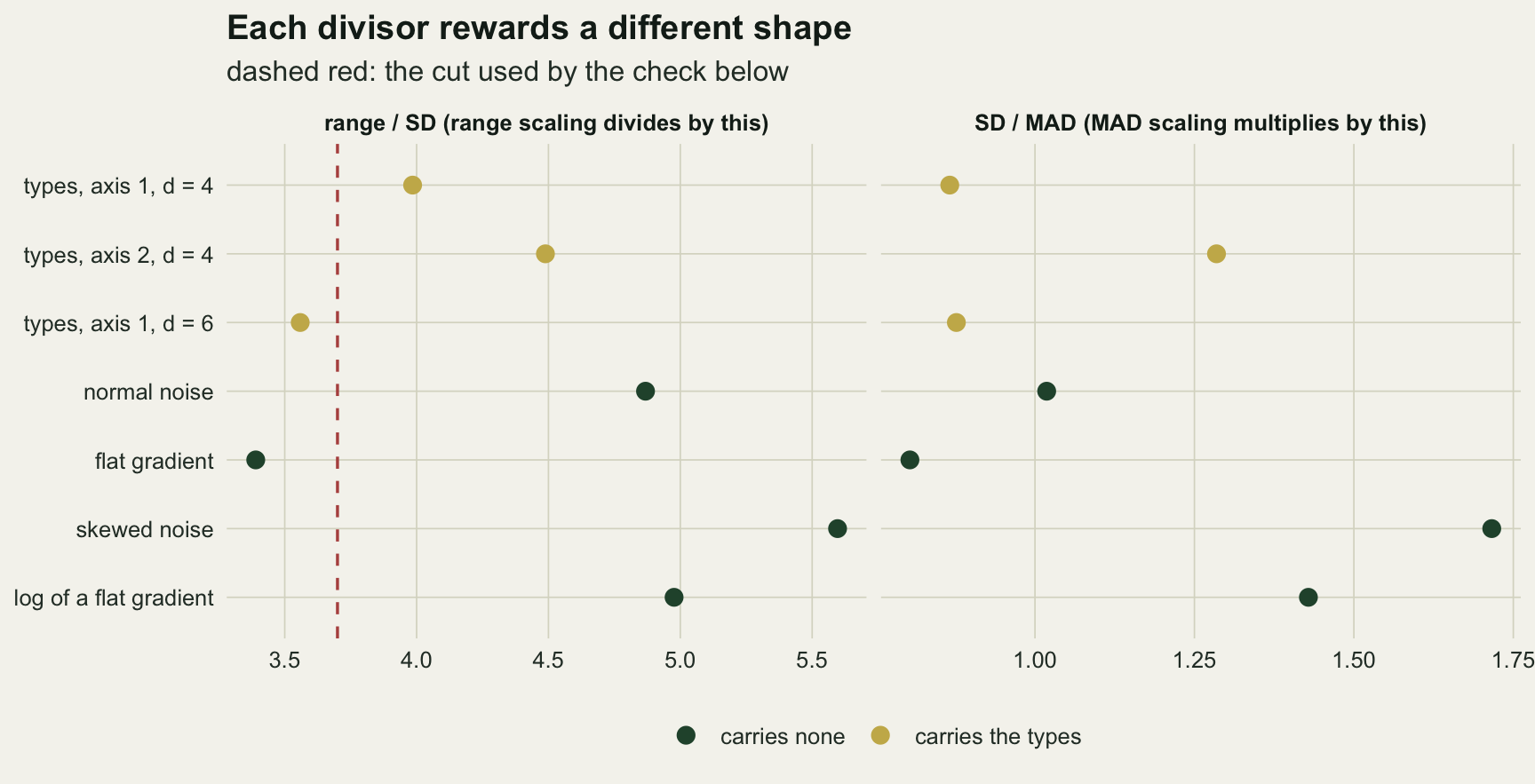
One extreme site, balanced types and the log transformation
The remaining cells change one thing at a time. The outlier arm adds eight standard deviations to one site on an informative variable. The balanced arm uses types of 27, 27 and 26. The single-variable arm keeps only one uninformative variable. The two log arms take the mixed cell and log either the two skewed variables only, which is what most analysts would do, or all four uninformative variables, including the flat gradients.
c4n_o <- cell_of(4, "normal", TRUE);  c3n_o <- cell_of(3, "normal", TRUE)
c4u_o <- cell_of(4, "uniform", TRUE); c4l_o <- cell_of(4, "lognormal", TRUE)
bal_n <- cell_of(4, "normal", arm_name = "balanced")
bal_u <- cell_of(4, "uniform", arm_name = "balanced")
one_n <- cell_of(4, "normal", arm_name = "one variable")
one_u <- cell_of(4, "uniform", arm_name = "one variable")
log_s <- cell_of(4, "mixed", arm_name = "log skewed only")
log_a <- cell_of(4, "mixed", arm_name = "log all four")
n_range_wins <- sum(cell_med$r_minus_z > 0)
One extreme site takes away most of what range scaling gained, because the range of the variable it sits on is now set by a single value. Under normal noise at a separation of four the gain of range over z falls from +0.222 to +0.016 (draws -0.007 to +0.053), and at a separation of three it becomes -0.047. The median and MAD, the usual answer to outliers, do not rescue the clustering: at a separation of four they score 0.283 against 0.409 for the z-score, the lowest of the three, and at three the difference from z is +0.004, with draws from -0.039 to +0.053. With flat gradients the outlier changes nothing about the verdict; range scaling was already failing.
Balancing the types does not remove the reversal. With 27, 27 and 26 sites, range minus z is +0.187 under normal noise and -0.346 under flat gradients. Reducing the uninformative variables to one shrinks the gain under normal noise to +0.027 and sharpens the loss under a flat gradient to -0.443: with a single empty variable the z-score scores 0.788, within 0.073 of the oracle, while range scaling reaches 0.316. One flat gradient given the largest weight is enough to cut the partition along it.
The log arms answer the question a numerical ecologist asks first. Logging the two skewed variables, the ordinary treatment of nutrient data, makes them normal and leaves the flat gradients alone, and range scaling still fails: 0.107 against 0.372. The MAD, freed from the skewed variables, comes up to 0.357. Logging all four, including the gradients, turns a flat gradient into a left-skewed variable with a long lower tail (its range-to-SD ratio is 4.98), and range scaling wins again, 0.625 against 0.450. The transformation matters because it changes shapes, and shapes are what the divisor reads. Logging an altitude or a depth that was laid out at even steps is not usually done, so the first log arm is the realistic one.
Across all 22 cells, range scaling beats the z-score in 10. Every cell where it loses contains a flat gradient that was not logged, or the outlier at the smaller separation.
cell_lab <- with(cells, paste0(
  "d ", d_sep, ", ", shape_lab[shape],
  ifelse(outlier, ", one outlier", ""),
  ifelse(arm == "grid", "", paste0(" (", arm, ")"))))
cell_lab[cells$arm == "one variable"] <- paste0("d 4, one ", c("normal noise", "flat gradient"),
                                                " variable only")
cells_df <- data.frame(lab = cell_lab, diff = cell_med$r_minus_z,
                       lo_d = cell_lo$r_minus_z, hi_d = cell_hi$r_minus_z,
                       check = ifelse(cell_med$pick_z > 0.5, "check chooses z-score",
                                      "check chooses range"))
cells_df$lab <- factor(cells_df$lab, levels = cells_df$lab[order(cells_df$diff)])

ggplot(cells_df, aes(diff, lab, colour = check)) +
  geom_vline(xintercept = 0, colour = te_body, linewidth = 0.5) +
  geom_errorbar(aes(xmin = lo_d, xmax = hi_d), orientation = "y", width = 0.3,
                linewidth = 0.5) +
  geom_point(size = 2.4) +
  scale_colour_manual(values = c(te_gold, te_forest), name = NULL) +
  labs(x = "range minus z-score (adjusted Rand index)", y = NULL,
       title = "Where range scaling pays and where it costs") +
  theme_datasheet() +
  theme(legend.position = "bottom")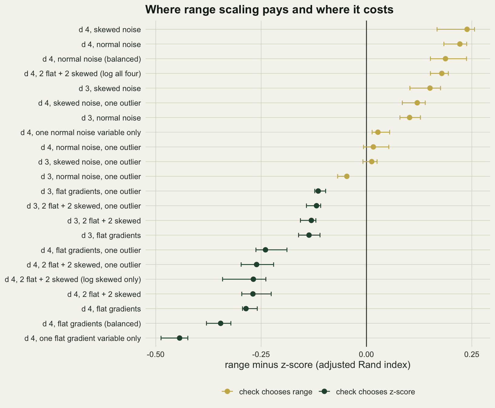
A check before choosing
The ratios suggest a check that needs nothing but the data: compute the range-to-SD ratio of every variable, and if any variable sits near the flat value (3.38 at eighty sites, the square root of 12 in large samples), do not divide by the range. The version scored here was written down before the grid ran: use the z-score if any variable has a ratio below 3.7, otherwise use range scaling. The MAD is left out of the check on purpose, because the grid shows that two skewed variables among four are enough to ruin it (0.111 in the mixed cell, 0.357 once those two are logged).
mean_sc <- colMeans(all_sets[, c("z", "range", "mad", "vr_weight", "rule", "oracle")])
d_rz <- all_sets$rule - all_sets$z
d_rr <- all_sets$rule - all_sets$range
se_rz <- sd(d_rz) / sqrt(length(d_rz))
se_rr <- sd(d_rr) / sqrt(length(d_rr))
pick_range_normal <- 1 - med(c4n, "pick_z")
flat_cell <- cells$shape %in% c("uniform", "mixed") & cells$log_what != "all"
flat_set  <- flat_cell[all_sets$cell]
n_flat_cells <- sum(flat_cell)
rz_flat <- mean(d_rz[flat_set]);  rz_other <- mean(d_rz[!flat_set])
rr_flat <- mean(d_rr[flat_set]);  rr_other <- mean(d_rr[!flat_set])

best_in_cell <- pmax(cell_med$z, cell_med$range, cell_med$mad)
regret <- c(z = max(best_in_cell - cell_med$z), range = max(best_in_cell - cell_med$range),
            mad = max(best_in_cell - cell_med$mad),
            rule = max(best_in_cell - cell_med$rule))

ward_cells <- which(cells$d_sep == 4)
ward_med <- t(vapply(ward_cells, function(i) {
  p <- per_set[[i]]
  dm <- aggregate(cbind(z, range, mad, ward_z, ward_range, ward_mad) ~ draw, p, mean)
  apply(dm[, -1], 2, median)
}, numeric(6)))
km_best   <- apply(ward_med[, c("z", "range", "mad")], 1, which.max)
ward_best <- apply(ward_med[, c("ward_z", "ward_range", "ward_mad")], 1, which.max)
ward_same_best <- sum(km_best == ward_best)
ward_same_sign <- sum(sign(ward_med[, "range"] - ward_med[, "z"]) ==
                      sign(ward_med[, "ward_range"] - ward_med[, "ward_z"]))
n_ward <- length(ward_cells)
Over all 6600 data sets, with every cell weighted equally, the mean index is 0.357 for always using the z-score, 0.291 for always using the range, 0.275 for always using the MAD, and 0.402 for the check. The check beats always-z by 0.046 (Monte Carlo standard error 0.002, paired over data sets) and always-range by 0.111 (standard error 0.003). It is not perfect. Under normal noise at a separation of four it chooses range scaling in only 78 per cent of data sets, because an informative variable or a noise variable occasionally dips below the cut by chance, and each such data set is clustered on z-scores and gives up part of the range’s gain.
A second way to read the grid is by the worst case. In each cell take the best of the three scalers, and ask how far each strategy falls below it in its worst cell. The z-score falls at most 0.349 below the best, the check 0.349, range scaling 0.599 and the MAD 0.676. The worst case for the z-score and for the check is a flat-gradient cell where the MAD does best; range scaling and the MAD each have a cell where they lose most of what the best scaler reached.
Ward’s method tells the same story as k-means. In the 14 cells at a separation of four, the sign of range minus z agrees between the two methods in 14 and the best of the three scalers is the same in 12.
The simplified variance-to-range weighting does not rescue the mixed cell. It scores 0.058 there, below all three plain scalers, and 0.278 over the whole grid. That is the arithmetic of the previous section again: after range scaling a flat gradient has the largest variance-to-range ratio of any shape in the grid at this separation, so weighting by that ratio gives it still more weight. Steinley and Brusco’s procedure pairs the weighting with a selection step that this version omits, so the result speaks against the shortcut and not against their method. What the oracle shows is the size of the prize for getting selection right: 0.766 over the grid, against 0.402 for the best scaling strategy.
What to report
Say which divisor was used and why, in the methods, not only that the variables were standardised. “Standardised” can mean any of the three scalers above, and in one and the same cell (skewed noise at a separation of four) their typologies agreed with the truth anywhere from 0.712 for range scaling down to 0.036 for the MAD.
Print the range-to-SD ratio of every variable next to the summary statistics. It costs one line (apply(x, 2, function(v) diff(range(v)) / sd(v))), it shows which variables are flat and which are long-tailed, and it is the whole reason the choice of divisor matters. At eighty sites, a variable near 3.4 to 3.5 is either an evenly spread gradient or a variable with well-separated groups, so look at its histogram before blaming the design; a variable well above 5 has a long tail that a MAD will blow up.
If the check says range scaling is safe, run the clustering both ways anyway and report how far the two typologies agree, as an adjusted Rand index between the two partitions. When they disagree, the variable shapes are the reason, and the ratios say which variables drove it. When nothing is known about the shapes, the z-score is the choice whose worst loss in this grid was the smallest.
Report any log transformation before the scaling step, with the variables it was applied to. Logging changes the shapes, and the log arms above show it can flip which scaler wins.
Honest limits
The informative variables here are always a mixture of normal groups, and the types differ only in their means on two variables. Real site types also differ in spread, and a type that is more variable than the others changes both ratios in ways this grid does not cover. The separations of three and four within-type standard deviations are moderate on purpose; at larger separations the differences between scalers should narrow, but this grid does not measure how fast. The check has the opposite problem at large separations: an informative variable with groups far apart has a range-to-SD ratio heading towards the flat limit, and the check would then refuse range scaling in exactly the case where it helps.
The average score of the check depends on the grid, and the grid is mine. In 11 of its 22 cells the uninformative variables include flat gradients that were not logged, which is more than a typical survey has. The check’s margin over always-z comes from the other cells (a mean gain of +0.093 there, against -0.001 in the flat-gradient cells), and its margin over always-range comes from the flat-gradient cells (+0.237 there, against -0.015 elsewhere). On a grid dominated by bell-shaped noise the margin over always-z would grow, while the margin over always-range would vanish and even turn slightly negative, since in the other cells the check trails always-range. What the check buys over always-range is insurance against flat gradients, and the worst-case reading is the more portable one.
The target is a crisp known typology, and the adjusted Rand index rewards only that. Real vegetation or lake types are not crisp: sites grade into each other, and a typology can be useful when it is only partly recoverable from environment. The index is still the right yardstick for comparing scalers on the same data, because the scaler is the only thing that changes, but its absolute values should not be read as the reliability of any real classification. The next step for a real typology is to ask whether it exceeds what clustering finds in structureless data, which is what checking a community classification does.
The weighting arm is a simplified stand-in for Steinley and Brusco’s procedure, and it omits their selection step. The oracle shows that dropping the empty variables would beat every scaler by a wide margin; variable selection in clustering, the problem Fowlkes, Gnanadesikan and Kettenring set out in 1988, is the real repair when variables that carry no groups are suspected, and it is not tested here.
Every cell uses k-means with three clusters, the true number. Choosing the number of clusters is a separate decision, and the divisor influences it too, since the empty variables that dominate a badly scaled distance can make a different number of clusters look natural.
References
Milligan GW, Cooper MC 1988 Journal of Classification 5(2):181-204 (10.1007/BF01897163)
Steinley D, Brusco MJ 2008 Multivariate Behavioral Research 43(1):77-108 (10.1080/00273170701836695)
Hubert L, Arabie P 1985 Journal of Classification 2(1):193-218 (10.1007/BF01908075)
Gower JC 1971 Biometrics 27(4):857-871 (10.2307/2528823)
Fowlkes EB, Gnanadesikan R, Kettenring JR 1988 Journal of Classification 5(2):205-228 (10.1007/BF01897164)