library(ggplot2)
library(patchwork)

te_paper  <- "#f5f4ee"
te_ink    <- "#16241d"
te_body   <- "#2c3a31"
te_forest <- "#275139"
te_rust   <- "#b5534e"
te_gold   <- "#c9b458"
te_line   <- "#dad9ca"

theme_datasheet <- function() {
  theme_minimal(base_size = 12) +
    theme(plot.background  = element_rect(fill = te_paper, colour = NA),
          panel.background = element_rect(fill = te_paper, colour = NA),
          panel.grid.major = element_line(colour = te_line, linewidth = 0.3),
          panel.grid.minor = element_blank(),
          text             = element_text(colour = te_body),
          plot.title       = element_text(colour = te_ink, face = "bold"),
          plot.subtitle    = element_text(colour = te_body),
          axis.text        = element_text(colour = te_body))
}Spatial sorting: the front that breeds its speed
R
invasion ecology
dispersal
evolutionary ecology
simulation
ecology tutorial
Simulate spatial sorting in R: a heritable dispersal trait accelerates an invasion front, and only the trait cline separates it from a fat-tailed kernel.
A cane toad caught at the leading edge of the Australian invasion covers more ground in a night than one caught in the long occupied country behind it, and its offspring do too. That single sentence breaks an assumption built into most spread models on this site and in most management plans: that the dispersal kernel is a fixed property of the species. If the individuals that arrive first are the ones that move furthest, and if moving far is heritable, then the front is not just a place where the population happens to be. It is a filter that concentrates a trait, and the filter runs again every generation.
The name for this is spatial sorting, and it is not a hypothesis on the site. Shine, Brown and Phillips named and demonstrated it in toads, Phillips and colleagues built the evolving-kernel theory, and two flour-beetle experiments, one by Ochocki and Miller and one by Weiss-Lehman and colleagues, showed that populations allowed to evolve spread both faster and more erratically than populations where the trait was shuffled between generations. This post is a demonstration of that published result, not a claim to it. What is measured here is narrower: how large the acceleration actually is as a function of the trait cline the front builds, whether the extent series alone can tell spatial sorting from a fat-tailed kernel, and what the dispersal cost term does to both answers.
The invasion posts already on the site all hold the kernel fixed and let its shape do the work. Fat tails and accelerating spread puts the acceleration in the tail of the kernel and fits a power of time to the resulting front, and its section on that fit is the instrument used again here. The speed of an invasion front derives the constant speed of a thin-tailed pulled front and shows the far tail of a Gaussian is genuinely irrelevant to it. Long-distance jumps and stratified spread shows that rare jumps lift the mean advance by a factor of about two and blow up the replicate-to-replicate variance by nearly ten. In all three the individuals are interchangeable. Here the kernel is Gaussian and its shape never changes; what changes is which individuals are carrying it.
The arithmetic core is elsewhere too. The breeder’s equation in R is the one-generation response to truncation selection, mid-parent inheritance plus a segregation term, and that is exactly the genetic engine used below. What this post adds is the selection event: at a moving front the truncation is done by geography, not by a breeder, and the cut is applied again from a new position every generation.
A corridor where the step length is inherited
The model is a one-dimensional corridor of 400 cells with a reflecting wall at the left end and an absorbing one at the right, seeded with a population filling the first ten cells at carrying capacity. No replicate of the main grid reaches the right-hand end; the deliberate no-cost arm does, and one comparison kernel needs a longer corridor and is given one. Each cell has Beverton-Holt density regulation with a capacity of 50 and a maximum per-parent output of 3. Every individual carries a dispersal trait, the standard deviation in cells of its own Gaussian step, and that trait is inherited on the log scale by the mid-parent rule plus a segregation term of half the genetic variance, with a fresh environmental deviation drawn each generation. Mating is with a random individual from the same cell, which is what makes the selection spatial: at the leading edge the only available mates are the other individuals that got there.
Heritability enters as the genetic share of a fixed total trait variance. Setting h2 to zero leaves the total variance intact, so the population is still a mixture of individuals with different step lengths, but none of that difference passes to the next generation. That arm is the control, and it is the one that decides whether anything below is evolution rather than a kernel mixture.
The last ingredient is a cost. Long moves are dangerous, so survival of a move of length d is exp(-m d). Without it the model has no brake at all, which is shown in its own section further down. The values of m and of the trait variance are the two knobs that set how steep a cline the front can build, and they are fixed before any run below.
n_cell <- 400L
cap_cell <- 50
r_max <- 3
n_gen <- 40L
seed_cells <- 10L
edge_band <- 10L

run_one <- function(h2, v_tot, m_cost, fat_df = NA, fat_scale = NA,
                    keep_profile = FALSE, cells = n_cell) {
  v_gen <- h2 * v_tot
  v_env <- (1 - h2) * v_tot
  pos <- rep(seq_len(seed_cells), each = cap_cell)
  g_val <- rnorm(length(pos), 0, sqrt(v_gen))
  e_val <- rnorm(length(pos), 0, sqrt(v_env))
  front <- numeric(n_gen)
  move_front <- NA_real_
  move_core <- NA_real_
  move_front_s <- NA_real_
  move_core_s <- NA_real_
  profile <- NULL
  for (tt in seq_len(n_gen)) {
    occ <- tabulate(pos, cells)
    fec <- r_max / (1 + (r_max - 1) * occ[pos] / cap_cell)
    n_off <- rpois(length(pos), fec)
    mum <- rep(seq_along(pos), n_off)
    if (length(mum) == 0L) break
    ord <- order(pos)
    cell_start <- c(1L, cumsum(occ)[-cells] + 1L)
    dad <- ord[cell_start[pos[mum]] + floor(runif(length(mum)) * occ[pos[mum]])]
    g_off <- (g_val[mum] + g_val[dad]) / 2 + rnorm(length(mum), 0, sqrt(v_gen / 2))
    e_off <- rnorm(length(mum), 0, sqrt(v_env))
    trait <- exp(g_off + e_off)
    move <- if (is.na(fat_df)) rnorm(length(mum), 0, trait) else
      fat_scale * rt(length(mum), fat_df)
    new_pos <- round(pos[mum] + move)
    new_pos <- ifelse(new_pos < 1L, 2L - new_pos, new_pos)
    alive <- new_pos <= cells & runif(length(new_pos)) < exp(-m_cost * abs(move))
    if (tt == n_gen) {
      home <- pos[mum]
      at_edge <- home >= max(home) - edge_band
      at_core <- home <= min(home) + edge_band
      move_front <- mean(abs(move[at_edge]))
      move_core <- mean(abs(move[at_core]))
      move_front_s <- mean(abs(move[at_edge & alive]))
      move_core_s <- mean(abs(move[at_core & alive]))
      if (keep_profile) profile <- data.frame(home = home, trait = trait, moved = abs(move))
    }
    pos <- new_pos[alive]
    g_val <- g_off[alive]
    e_val <- e_off[alive]
    if (length(pos) == 0L) break
    front[tt] <- max(pos)
  }
  gen_fit <- 10:n_gen
  list(front = front, extent = front[n_gen],
       early = (front[15] - front[6]) / 9,
       late = (front[40] - front[31]) / 9,
       b = coef(lm(log(pmax(front[gen_fit] - seed_cells, 0.5)) ~ log(gen_fit)))[[2]],
       move_front = move_front, move_core = move_core,
       move_front_s = move_front_s, move_core_s = move_core_s,
       wall_gen = if (any(front >= cells - 1)) which(front >= cells - 1)[1] else NA_integer_,
       profile = profile)
}
Four numbers come out of each replicate. The early speed is the average cell gain per generation over generations 6 to 15, the late speed the same over generations 31 to 40, and their ratio is the acceleration. The exponent b is the slope of log front position on log generation over generations 10 to 40, measuring the front from the edge of the seeded block, which is the fit used in the fat-tails post and for the same reason: an additive offset otherwise drags the exponent below one even for a straight line. The cline is the mean absolute realised move of the offspring born in the leading ten cells divided by the same quantity in the trailing ten cells, which is what a field study measures when it radio-tracks animals at the front and in the core. It is the attempted step: offspring that the cost then kills are counted in it, and the survivors-only version is reported alongside it further down.
n_rep_grid <- 60L

run_arm <- function(arm, h2, v_tot, m_cost, n_rep = n_rep_grid, fat_df = NA,
                    fat_scale = NA, cells = n_cell) {
  rr <- lapply(seq_len(n_rep), function(i)
    run_one(h2, v_tot, m_cost, fat_df, fat_scale, cells = cells))
  list(per_rep = data.frame(arm = arm, h2 = h2, v_tot = v_tot, m_cost = m_cost,
         rep = seq_len(n_rep), extent = sapply(rr, `[[`, "extent"),
         early = sapply(rr, `[[`, "early"), late = sapply(rr, `[[`, "late"),
         b = sapply(rr, `[[`, "b"), move_front = sapply(rr, `[[`, "move_front"),
         move_core = sapply(rr, `[[`, "move_core"),
         move_front_s = sapply(rr, `[[`, "move_front_s"),
         move_core_s = sapply(rr, `[[`, "move_core_s"),
         wall_gen = sapply(rr, `[[`, "wall_gen")),
       fronts = sapply(rr, `[[`, "front"))
}

arm_summary <- function(pr) {
  boot_ratio <- replicate(2000, {
    idx <- sample(nrow(pr), nrow(pr), replace = TRUE)
    mean(pr$late[idx]) / mean(pr$early[idx])
  })
  data.frame(arm = pr$arm[1], h2 = pr$h2[1], v_tot = pr$v_tot[1], m_cost = pr$m_cost[1],
    extent = mean(pr$extent), sd_extent = sd(pr$extent),
    early = mean(pr$early), late = mean(pr$late),
    ratio = mean(pr$late) / mean(pr$early), ratio_se = sd(boot_ratio),
    b = mean(pr$b), b_se = sd(pr$b) / sqrt(nrow(pr)),
    cline = mean(pr$move_front / pr$move_core),
    cline_surv = mean(pr$move_front_s / pr$move_core_s),
    cv_extent = sd(pr$extent) / mean(pr$extent),
    walls = sum(!is.na(pr$wall_gen)))
}

settings <- data.frame(v_tot = c(0.20, 0.05, 0.05), m_cost = c(0.05, 0.20, 0.05))
h2_grid <- c(0, 0.1, 0.25, 0.5)
set.seed(4271)
arms <- list()
for (s in seq_len(nrow(settings))) {
  for (h in h2_grid) {
    lab <- sprintf("s%d_h%03.0f", s, 100 * h)
    arms[[lab]] <- run_arm(lab, h, settings$v_tot[s], settings$m_cost[s])
  }
}
sorting_tab <- do.call(rbind, lapply(arms, function(a) arm_summary(a$per_rep)))
n_rep_used <- nrow(arms[[1]]$per_rep)
sd_rel_unc <- 1 / sqrt(2 * (n_rep_used - 1))
print(round(sorting_tab[, c("h2", "v_tot", "m_cost", "extent", "sd_extent",
                            "ratio", "b", "cline")], 3))
h2 v_tot m_cost extent sd_extent ratio b cline
s1_h000 0.00 0.20 0.05 75.233 4.382 1.007 0.944 1.008
s1_h010 0.10 0.20 0.05 110.233 23.976 1.650 1.190 2.185
s1_h025 0.25 0.20 0.05 172.100 33.871 2.628 1.457 7.351
s1_h050 0.50 0.20 0.05 263.750 39.905 2.359 1.646 14.265
s2_h000 0.00 0.05 0.20 55.967 2.940 1.005 0.928 1.008
s2_h010 0.10 0.05 0.20 60.267 5.554 1.092 0.978 1.187
s2_h025 0.25 0.05 0.20 62.533 9.021 1.164 0.998 1.458
s2_h050 0.50 0.05 0.20 69.283 10.511 1.318 1.072 1.951
s3_h000 0.00 0.05 0.05 63.133 2.925 0.968 0.947 1.005
s3_h010 0.10 0.05 0.05 70.517 6.619 1.180 1.013 1.265
s3_h025 0.25 0.05 0.05 82.067 13.205 1.349 1.095 1.665
s3_h050 0.50 0.05 0.05 102.200 21.793 2.013 1.278 2.962Twelve arms, 60 replicates each, 40 generations: three trait-variance and cost settings crossed with four heritabilities. The whole grid runs in well under a minute because everything inside a generation is vectorised over individuals.
traj_of <- function(lab, tag) {
  fr <- arms[[lab]]$fronts
  data.frame(gen = rep(seq_len(n_gen), ncol(fr)),
             front = as.vector(fr),
             rep = rep(seq_len(ncol(fr)), each = n_gen),
             arm = tag)
}
traj <- rbind(traj_of("s1_h000", "h2 = 0"), traj_of("s1_h025", "h2 = 0.25"),
              traj_of("s1_h050", "h2 = 0.5"))
traj$arm <- factor(traj$arm, levels = c("h2 = 0", "h2 = 0.25", "h2 = 0.5"))

set.seed(9014)
prof_runs <- lapply(c(0, 0.25, 0.5), function(h)
  run_one(h, settings$v_tot[1], settings$m_cost[1], keep_profile = TRUE))
prof <- do.call(rbind, Map(function(z, h) {
  pf <- z$profile
  pf$bin <- cut(pf$home, breaks = seq(0, n_cell, by = 20), labels = FALSE)
  agg <- aggregate(moved ~ bin, pf, mean)
  agg$cell <- 20 * agg$bin - 10
  agg$arm <- sprintf("h2 = %s", h)
  agg
}, prof_runs, c(0, 0.25, 0.5)))
prof$arm <- factor(prof$arm, levels = c("h2 = 0", "h2 = 0.25", "h2 = 0.5"))
arm_cols <- c("h2 = 0" = te_rust, "h2 = 0.25" = te_gold, "h2 = 0.5" = te_forest)
p_traj <- ggplot(traj, aes(gen, front, group = interaction(arm, rep), colour = arm)) +
geom_line(linewidth = 0.3, alpha = 0.6) +
scale_colour_manual(values = arm_cols, name = NULL) +
labs(x = "Generation", y = "Front position (cells)",
title = "Replicate fronts") +
guides(colour = guide_legend(override.aes = list(linewidth = 0.9, alpha = 1))) +
theme_datasheet() + theme(legend.position = "bottom")
p_prof <- ggplot(prof, aes(cell, moved, colour = arm)) +
geom_line(linewidth = 0.7) +
geom_point(size = 1.3, show.legend = FALSE) +
scale_colour_manual(values = arm_cols, name = NULL) +
labs(x = "Position in corridor (cells)", y = "Mean realised move (cells)",
title = "The cline at generation 40") +
guides(colour = guide_legend(override.aes = list(linewidth = 0.9, alpha = 1))) +
theme_datasheet() + theme(legend.position = "bottom")
(p_traj | p_prof) +
plot_layout(guides = "collect") +
plot_annotation(theme = theme_datasheet()) &
theme(legend.position = "bottom")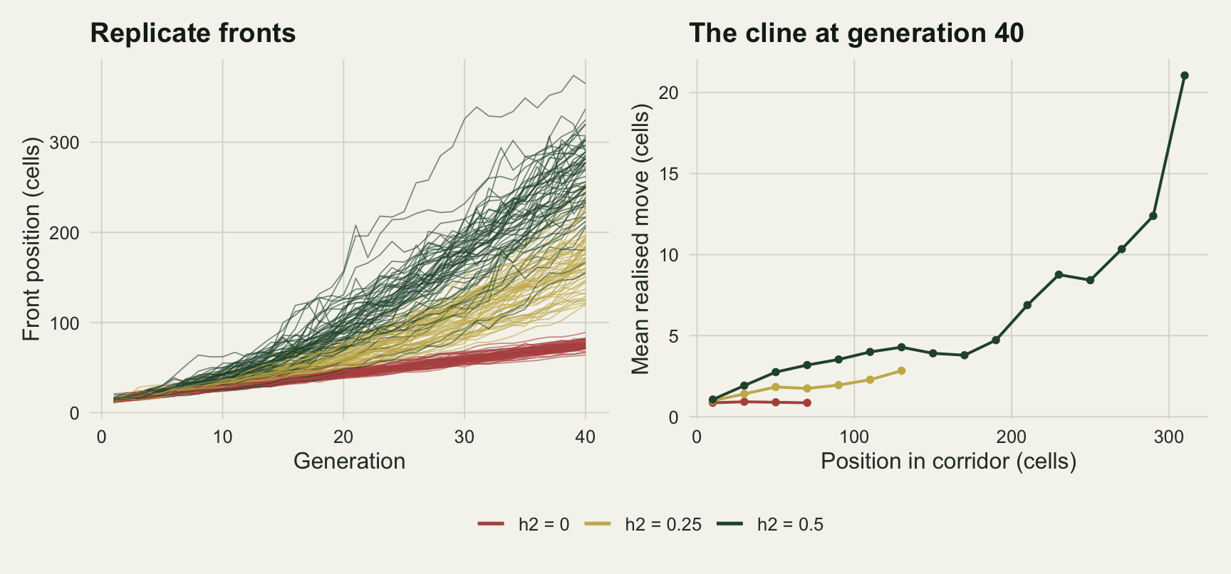
The control: a mixture of kernels is not evolution
The three zero-heritability arms keep the full spread of individual step lengths and destroy only the inheritance. If the acceleration came from the mixture of kernels, from the fact that some individuals simply move further than others, these arms would accelerate too.
ctrl <- sorting_tab[sorting_tab$h2 == 0, ]
ctrl_ratio_lo <- min(ctrl$ratio)
ctrl_ratio_hi <- max(ctrl$ratio)
ctrl_b_lo <- min(ctrl$b)
ctrl_b_hi <- max(ctrl$b)
ctrl_cline_lo <- min(ctrl$cline)
ctrl_cline_hi <- max(ctrl$cline)
ctrl_sd_lo <- min(ctrl$sd_extent)
ctrl_sd_hi <- max(ctrl$sd_extent)
ctrl_ratio_se <- max(ctrl$ratio_se)
print(round(ctrl[, c("v_tot", "m_cost", "extent", "sd_extent", "ratio",
                     "ratio_se", "b", "cline")], 3))
v_tot m_cost extent sd_extent ratio ratio_se b cline
s1_h000 0.20 0.05 75.233 4.382 1.007 0.032 0.944 1.008
s2_h000 0.05 0.20 55.967 2.940 1.005 0.029 0.928 1.008
s3_h000 0.05 0.05 63.133 2.925 0.968 0.027 0.947 1.005They do not. Across the three control arms the speed ratio runs from 0.97 to 1.01, with a bootstrap standard error of at most 0.03, so none of them is distinguishable from a constant speed. The log-log exponent runs from 0.93 to 0.95, that is, just under one, which is what the fat-tails post reports for a Gaussian front still converging upwards on its asymptotic speed. The measured cline is 1.00 to 1.01, so individuals at the front move as far as individuals at the back to within a few per cent, because the trait is redrawn from the same distribution every generation wherever you stand. The standard deviation of the final extent across replicates is 2.9 to 4.4 cells.
That last number is the denominator for everything that follows. A standard deviation estimated from 60 replicates carries a relative uncertainty of about 9 per cent, so variance ratios below about one and a half should not be read as real.
Three signatures against one axis
With inheritance switched on, the interesting question is not whether the front accelerates but by how much, and the honest answer is that there is no single number. The acceleration is set by the trait cline the front manages to build, and the cline is set by how much trait variance there is and how expensive long moves are. So the three settings and four heritabilities are plotted against the cline they produce rather than against h2.
sorting_tab$sd_ratio <- NA_real_
for (i in seq_len(nrow(sorting_tab))) {
  base <- sorting_tab$sd_extent[sorting_tab$v_tot == sorting_tab$v_tot[i] &
                                sorting_tab$m_cost == sorting_tab$m_cost[i] &
                                sorting_tab$h2 == 0]
  sorting_tab$sd_ratio[i] <- sorting_tab$sd_extent[i] / base
}
field_row <- sorting_tab[sorting_tab$v_tot == 0.05 & sorting_tab$m_cost == 0.20 &
                         sorting_tab$h2 == 0.5, ]
alt_row <- sorting_tab[sorting_tab$v_tot == 0.20 & sorting_tab$m_cost == 0.05 &
                       sorting_tab$h2 == 0.1, ]
mid_row <- sorting_tab[sorting_tab$v_tot == 0.05 & sorting_tab$m_cost == 0.05 &
                       sorting_tab$h2 == 0.5, ]
peak_row <- sorting_tab[sorting_tab$v_tot == 0.20 & sorting_tab$m_cost == 0.05 &
                        sorting_tab$h2 == 0.25, ]
top_row <- sorting_tab[sorting_tab$v_tot == 0.20 & sorting_tab$m_cost == 0.05 &
                       sorting_tab$h2 == 0.5, ]
evo <- sorting_tab[sorting_tab$h2 > 0, ]
slope_sum <- summary(lm(log(ratio) ~ log(cline), evo))
slope_fit <- coef(slope_sum)[2, 1]
slope_se <- coef(slope_sum)[2, 2]
slope_r2 <- slope_sum$r.squared
ctrl_cv <- ctrl$cv_extent[ctrl$v_tot == field_row$v_tot & ctrl$m_cost == field_row$m_cost]
cv_ratio_field <- field_row$cv_extent / ctrl_cv
b_top_gap <- top_row$b - peak_row$b
b_top_gap_se <- sqrt(top_row$b_se^2 + peak_row$b_se^2)
cline_drop <- 100 * (1 - field_row$cline_surv / field_row$cline)
walls_total <- sum(sorting_tab$walls)
n_rep_total <- n_rep_used * nrow(sorting_tab)
ratio_top_gap <- peak_row$ratio - top_row$ratio
ratio_top_gap_se <- sqrt(peak_row$ratio_se^2 + top_row$ratio_se^2)
print(round(sorting_tab[, c("h2", "v_tot", "m_cost", "cline", "ratio",
                            "b", "sd_ratio", "early", "late")], 3))
h2 v_tot m_cost cline ratio b sd_ratio early late
s1_h000 0.00 0.20 0.05 1.008 1.007 0.944 1.000 1.569 1.580
s1_h010 0.10 0.20 0.05 2.185 1.650 1.190 5.472 1.963 3.239
s1_h025 0.25 0.20 0.05 7.351 2.628 1.457 7.730 2.498 6.565
s1_h050 0.50 0.20 0.05 14.265 2.359 1.646 9.107 3.930 9.269
s2_h000 0.00 0.05 0.20 1.008 1.005 0.928 1.000 1.089 1.094
s2_h010 0.10 0.05 0.20 1.187 1.092 0.978 1.889 1.204 1.315
s2_h025 0.25 0.05 0.20 1.458 1.164 0.998 3.068 1.220 1.420
s2_h050 0.50 0.05 0.20 1.951 1.318 1.072 3.575 1.244 1.641
s3_h000 0.00 0.05 0.05 1.005 0.968 0.947 1.000 1.311 1.269
s3_h010 0.10 0.05 0.05 1.265 1.180 1.013 2.263 1.400 1.652
s3_h025 0.25 0.05 0.05 1.665 1.349 1.095 4.514 1.565 2.111
s3_h050 0.50 0.05 0.05 2.962 2.013 1.278 7.450 1.587 3.194Where the realistic end of that axis sits is a field question, and this post does not settle it. No published front-to-core contrast in individual dispersal was verified for this post. The toad study cited below reports a steady increase in dispersal tendency with distance from the origin, and a front speed that rose from about 10 kilometres a year to more than 55, but that is the speed of the front, not a ratio between individuals caught at the front and in the core. So the rows are labelled by their measured cline and by nothing else, and the two arms nearest a cline of two are the ones to read first.
Two arms land near a cline of two and they do not agree. One sits at 1.95 with a speed ratio of 1.32, the other at 2.19 with a ratio of 1.65 (bootstrap standard errors 0.06 and 0.09), so a cline of two does not fix an acceleration: the trait variance and the cost that produced the cline still matter. The first of the two is the one carried through the rest of the post, and picking the second instead would have changed the headline. At that arm the late speed is 1.32 times the early speed (bootstrap standard error 0.06), the log-log exponent is 1.07 with a standard error of 0.01, and the extent standard deviation is 3.6 times its own control. The arms at 7.4 and 14.3 are strong-cline rows a model can produce more easily than a field study can find.
Those three numbers say different things about the same run. An acceleration of 32 per cent between the two windows is real but not dramatic, and an exponent of 1.07, although 60 replicates separate it from one, sits below the range the fat-tails post measures for its fat kernels, so a single series of this shape would not send anyone looking for a tail. The variance signature, by contrast, is large: replicate extents spread 3.6 times as widely as under the control in absolute cells, which is well past the 9 per cent uncertainty on a standard deviation from 60 replicates. Part of that is a mean effect, because the evolving arm also travels further: on the coefficient of variation the same comparison is 2.9-fold. At a realistic cline the acceleration is modest and the unpredictability is what a manager would actually notice, which is the direction Ochocki and Miller report from their beetle experiment.
Push the cline harder and the acceleration arrives. At a cline of 3.0 the speed ratio is 2.01 and the exponent 1.28; at 7.4 the ratio is 2.63 and the exponent 1.46. Across the nine arms with non-zero heritability the speed ratio scales as the cline to the power 0.35, with a standard error of 0.06 and an R-squared of 0.84. The line accounts for most of the spread but not all of it, and the next paragraph shows where it fails. Taken as a direction rather than a law, it is the compact statement of the headline: the acceleration is a function of the cline, not a constant of the mechanism.
The scaling is not monotone at the top. The strongest arm, cline 14.3, gives a speed ratio of only 2.36, below the 2.63 of the arm one heritability step down. The reason is in the denominator, and the early speeds show it: 3.9 cells per generation in the strongest arm against 2.5 one heritability step down and 1.6 in the matching control, so by generation 6 the strongest arm’s early window is already measuring a fast front, while its late speeds differ far less (9.3 against 6.6). It is not the corridor wall either: 0 of the 720 replicates in the grid reach the far end. The drop itself is small against its own error, 0.27 with a combined bootstrap standard error of 0.18, so it is the flatness rather than the fall that is established. The exponent, which uses the whole trajectory rather than two windows, does not flatten at all: 1.65 against 1.46, a difference of 0.19 against a combined standard error of 0.03. Any single ratio quoted for spatial sorting therefore depends on where the early window was put.
set_lab <- c("Vtot 0.2, m 0.05", "Vtot 0.05, m 0.2", "Vtot 0.05, m 0.05")
sorting_tab$setting <- factor(set_lab[match(paste(sorting_tab$v_tot, sorting_tab$m_cost),
                                            paste(settings$v_tot, settings$m_cost))],
                              levels = set_lab)
set_cols <- c(te_forest, te_rust, te_gold)
names(set_cols) <- set_lab

sig_panel <- function(yvar, ylab, hline, ttl) {
  ggplot(sorting_tab, aes(cline, .data[[yvar]], colour = setting)) +
    geom_hline(yintercept = hline, linetype = 2, colour = te_body, linewidth = 0.3) +
    geom_point(size = 2.2) +
    scale_x_log10() +
    scale_colour_manual(values = set_cols, name = NULL) +
    labs(x = "Front / core move length", y = ylab, title = ttl) +
    theme_datasheet() + theme(legend.position = "bottom")
}
(sig_panel("ratio", "Late speed / early speed", 1, "Acceleration") |
 sig_panel("b", "Exponent b", 1, "Power of time") |
 sig_panel("sd_ratio", "SD relative to control", 1, "Replicate spread")) +
  plot_layout(guides = "collect") +
  plot_annotation(theme = theme_datasheet()) &
  theme(legend.position = "bottom")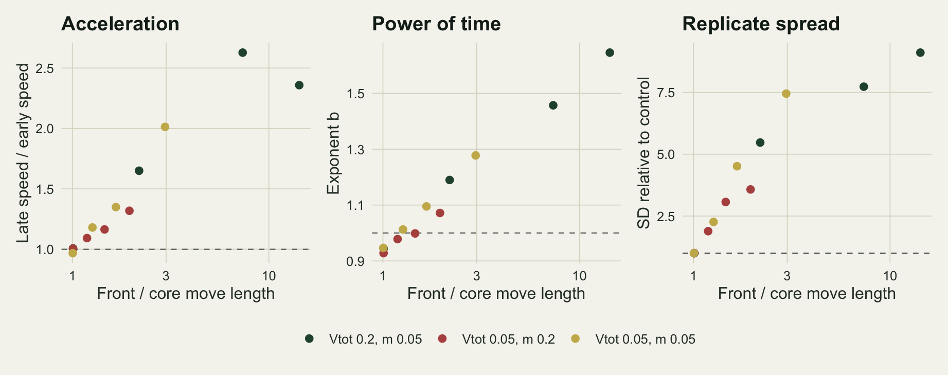
What the extent series cannot tell you
A spread modeller who is handed the front positions and nothing else will reach for the power-of-time fit from the fat-tails post, and an exponent above one is usually read as evidence for a fat kernel. The question is whether that reading can be wrong. The test is to run the same corridor with no heritable trait at all and a genuinely fat kernel instead: a Student t with two degrees of freedom, whose density falls off as the cube of distance.
Comparing two kernels means deciding what to hold equal, and that decision turns out to carry the answer. Two conventions are used here. The first matches the outcome: three t scales chosen from a short pre-run so that the mean extents land in the same range as the sorting arms. The second is the convention the fat-tails post uses, which gives every kernel the same median absolute displacement, so that the bulk of the dispersal is held fixed and only the far tail varies. Under both, the fat arms carry no dispersal cost, matching the way the fat-tails post’s model is built, so the comparison differs in kernel family and in the cost term as well as in scale.
set.seed(5507)
fat_scales <- c(0.15, 0.20, 0.25)
fat_arms <- lapply(fat_scales, function(sc)
  run_arm(sprintf("fat%03.0f", 100 * sc), 0, 0, 0, fat_df = 2, fat_scale = sc))
fat_tab <- do.call(rbind, lapply(fat_arms, function(a) arm_summary(a$per_rep)))
fat_tab$scale <- fat_scales
fat_b_lo <- min(fat_tab$b); fat_b_hi <- max(fat_tab$b)
fat_cline_lo <- min(fat_tab$cline); fat_cline_hi <- max(fat_tab$cline)
fat_sd_lo <- min(fat_tab$sd_extent); fat_sd_hi <- max(fat_tab$sd_extent)
pair_fat <- fat_tab[fat_tab$scale == 0.20, ]
pair_sort <- mid_row
b_gap <- pair_sort$b - pair_fat$b
b_gap_se <- sqrt(pair_fat$b_se^2 + pair_sort$b_se^2)
b_gap_field <- field_row$b - pair_fat$b
b_gap_field_se <- sqrt(pair_fat$b_se^2 + field_row$b_se^2)
kern_draws <- 2e5
sort_step <- abs(rnorm(kern_draws, 0,
                       exp(rnorm(kern_draws, 0, sqrt(pair_sort$v_tot)))))
fat_step <- abs(pair_fat$scale * rt(kern_draws, 2))
med_sort <- median(sort_step)
med_fat <- median(fat_step)
zero_sort <- mean(round(sort_step) == 0)
zero_fat <- mean(round(fat_step) == 0)
fat_ratios <- paste(sprintf("%.2f", fat_tab$ratio), collapse = ", ")
fat_ratio_se_lo <- min(fat_tab$ratio_se)
fat_ratio_se_hi <- max(fat_tab$ratio_se)
b_overlap <- mean(outer(fat_arms[[2]]$per_rep$b, arms[["s3_h050"]]$per_rep$b, ">"))
ratio_gap <- pair_sort$ratio - pair_fat$ratio
ratio_gap_se <- sqrt(pair_sort$ratio_se^2 + pair_fat$ratio_se^2)
print(round(fat_tab[, c("scale", "extent", "sd_extent", "ratio", "ratio_se",
                        "b", "b_se", "cline")], 3))
scale extent sd_extent ratio ratio_se b b_se cline
1 0.15 70.933 27.128 1.410 0.349 1.099 0.068 1.032
2 0.20 112.067 55.318 1.151 0.307 1.247 0.065 1.019
3 0.25 134.550 56.163 1.364 0.215 1.100 0.056 0.989Start with the pair matched on extent. The fat arm at scale 0.20 finishes at a mean of 112 cells and the sorting arm with a cline of 3.0 at 102 cells. Their exponents are 1.25 for the fat kernel and 1.28 for spatial sorting, a gap of 0.03 against a combined standard error of 0.07: the fit does not tell them apart even with 60 replicates on each side. Per replicate it is worse, as it must be: the fat arm’s exponent exceeds the sorting arm’s 44 per cent of the time. The two-window speed ratio does better in this one pair, 2.01 for sorting against 1.15 for the fat kernel, a gap of 0.86 against a combined standard error of 0.32, but the three fat scales give 1.41, 1.15, 1.36 with bootstrap standard errors of 0.22 to 0.35, a range that overlaps the sorting arms at field-scale clines, so that gap is a property of this pair and not a test.
Matching on extent is not matching on dispersal, and the price is paid in the bulk of the kernel. Drawn from the two kernels as they are specified, the sorting arm’s step has a median absolute length of 0.66 cells against 0.16 for the fat arm, and 87 per cent of the fat arm’s offspring round back into the cell they were born in, against 39 per cent for the sorting arm. Almost the whole fat population is standing still and the front moves only when a draw from the tail carries it, which is what the staircases in the figure below are. The obvious objection is that the comparison has been rigged by the scale, so the other convention is worth running.
set.seed(6142)
bulk_scale <- med_sort / qt(0.75, 2)
long_cells <- 4000L
bulk_arm <- run_arm("fatbulk", 0, 0, 0, fat_df = 2, fat_scale = bulk_scale,
                    cells = long_cells)
bulk_tab <- arm_summary(bulk_arm$per_rep)
bulk_over <- sum(apply(bulk_arm$fronts, 2, max) > n_cell)
print(round(c(scale = bulk_scale, extent = bulk_tab$extent,
              sd_extent = bulk_tab$sd_extent, ratio = bulk_tab$ratio,
              ratio_se = bulk_tab$ratio_se, b = bulk_tab$b, b_se = bulk_tab$b_se,
              cline = bulk_tab$cline, past_400_cells = bulk_over,
              reached_4000 = bulk_tab$walls), 3))
scale extent sd_extent ratio ratio_se
0.813 981.617 530.246 1.275 0.335
b b_se cline past_400_cells reached_4000
1.336 0.068 1.104 60.000 0.000 bulk_cline_se <- sd(bulk_arm$per_rep$move_front / bulk_arm$per_rep$move_core) /
sqrt(nrow(bulk_arm$per_rep))Giving the t kernel the same median absolute step as the sorting arm needs a scale of 0.81, four times the extent-matched one, and it changes the distance travelled out of all recognition: a mean extent of 982 cells against the sorting arm’s 102, with 60 of the 60 replicates past the 400-cell mark, which is why this arm is run in a corridor of 4000 cells. The sorting arms are unaffected by the corridor length, since none of them comes near 400. What barely changes is the exponent: 1.34 with a standard error of 0.07, against 1.25 for the same kernel matched on extent and 1.28 for spatial sorting. The two conventions disagree about how far the fat kernel goes by a factor of nearly ten and agree about the power of time to within their standard errors, which is the clearest evidence in the post that the exponent is not carrying information about the kernel here.
What does not discriminate is one exponent without a matched control. The fat arms give exponents from 1.10 to 1.25; the sorting arms with non-zero heritability give 0.98 to 1.65, a range that contains the whole fat range. The field-scale sorting arm sits at 1.07, which is 0.18 below the fat arm’s 1.25 against a combined standard error of 0.07: the exponent does order these two, in the direction opposite to the usual reading. An observed exponent between 1.10 and 1.25 is compatible with either mechanism.
Nor does the replicate spread. The fat arms’ extent standard deviations run from 27.1 to 56.2 cells and the sorting arms’ from 5.6 to 39.9; in the matched pair the fat arm is at 55 cells against the sorting arm’s 22, so on that axis the fat kernel is the more erratic of the two.
The cline does separate them, and it is the only quantity here that does cleanly. Across all three fat arms the measured front-to-core move ratio is 0.99 to 1.03, indistinguishable from the zero-heritability control, because every individual in those runs draws from the same kernel wherever it stands, and the bulk-matched arm gives 1.10, with a standard error of 0.18 because a mean of Student t steps is itself a noisy quantity. The sorting arm they are matched to has a cline of 3.0. That is a quantity you get by measuring animals, not by fitting the front, and it is the reason field studies of spatial sorting track individuals at the edge and in the core rather than mapping the range boundary faster.
series_of <- function(arm_obj, tag) {
  fr <- arm_obj$fronts
  gg <- 10:n_gen
  data.frame(gen = rep(gg, ncol(fr)),
             adv = as.vector(fr[gg, ]) - seed_cells,
             rep = rep(seq_len(ncol(fr)), each = length(gg)),
             arm = tag)
}
lab_sort <- sprintf("Spatial sorting, b = %.2f", pair_sort$b)
lab_fat <- sprintf("Fat kernel, extent matched, b = %.2f", pair_fat$b)
lab_bulk <- sprintf("Fat kernel, bulk matched, b = %.2f", bulk_tab$b)
ser <- rbind(series_of(arms[["s3_h050"]], lab_sort),
             series_of(fat_arms[[2]], lab_fat),
             series_of(bulk_arm, lab_bulk))
ser$arm <- factor(ser$arm, levels = c(lab_sort, lab_fat, lab_bulk))
ser <- ser[ser$adv > 0, ]
ggplot(ser, aes(gen, adv, group = rep)) +
  geom_line(linewidth = 0.35, alpha = 0.7, colour = te_forest) +
  facet_wrap(~ arm, nrow = 1) +
  scale_x_log10() + scale_y_log10() +
  labs(x = "Generation (log scale)", y = "Front beyond the seeded block (log scale)") +
  theme_datasheet() +
  theme(strip.text = element_text(colour = te_ink, face = "bold"))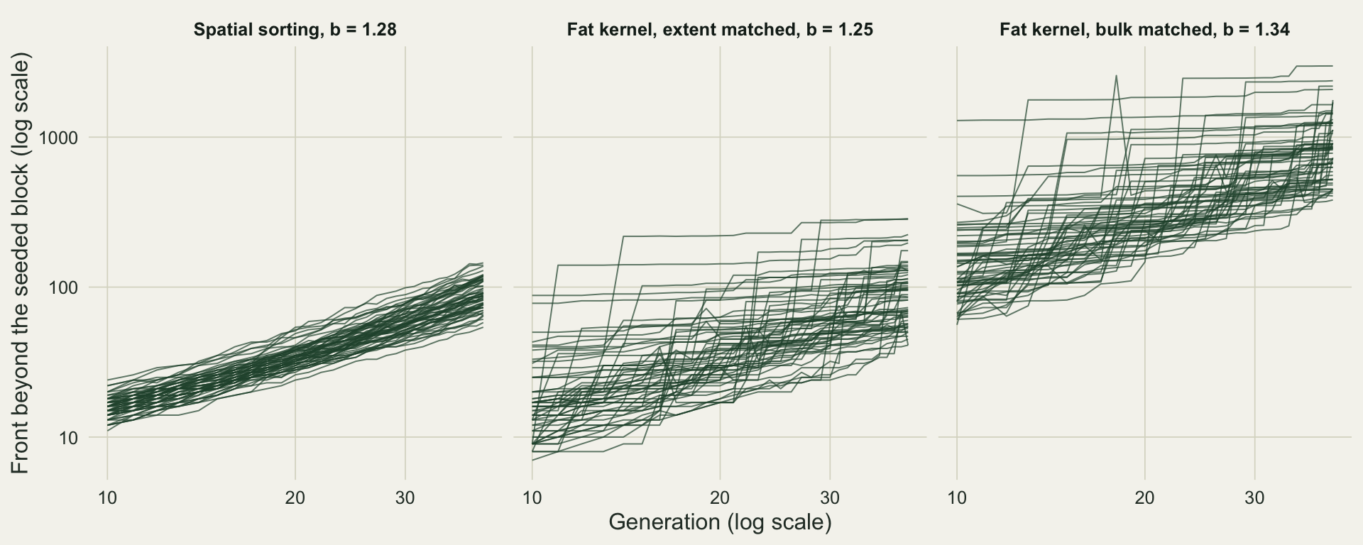
The figure adds a difference that is real but not usable on one invasion: the sorting replicates are a tight bundle of smooth curves, the fat-kernel replicates are staircases scattered over a wide band, under either matching. A manager watching a real invasion sees one of those lines, not the bundle, and one staircase with two flat decades in it is not distinguishable from one smooth curve with two bad survey years in it.
Without a dispersal cost the front leaves the map
Everything above carries a survival cost that falls with move length. That term is not decoration. Remove it and the sorting has no brake at all: each generation the furthest movers found the edge, their offspring inherit a longer step and pay nothing for it, and the trait ratchets until the corridor runs out.
set.seed(8821)
nocost <- run_arm("nocost", 0.5, 0.20, 0)
nocost_sum <- arm_summary(nocost$per_rep)
wall_gen_med <- median(nocost$per_rep$wall_gen)
wall_gen_min <- min(nocost$per_rep$wall_gen)
cost_row <- top_row
print(round(c(replicates = nrow(nocost$per_rep), reached_wall = nocost_sum$walls,
              first_wall_gen = wall_gen_min, median_wall_gen = wall_gen_med,
              cline = nocost_sum$cline), 2))
replicates reached_wall first_wall_gen median_wall_gen cline
60.00 60.00 19.00 28.50 15.94 All 60 replicates of the no-cost arm reach the far end of the 400-cell corridor, the first at generation 19 and the median at generation 28.5, while the same trait variance and heritability with a cost of 0.05 per cell finishes at 264 cells. Nothing about the no-cost run can be quoted as a speed, because the number that comes out is a property of the corridor length. Any spatial sorting model reported without its cost term is in that situation whether or not the wall is visible in the output.
The cost used here is mortality that rises with distance moved, which is the simplest form and the one with the clearest mechanism: a long move is time spent outside a territory. Perkins and colleagues let dispersal trade off against life history instead, and that choice changes the magnitudes, not the sign. The point for a reader is that the cost is a free parameter of any spatial sorting model, and the acceleration it permits is what your model reports.
What to report
A spread model with evolving dispersal needs four things stated before any speed can be interpreted.
The cost term comes first: its form (mortality per unit distance, or a fecundity trade-off), its magnitude, and what the run does without it. If every replicate hits the edge of the domain, the speed you measured is the domain’s.
The second is the cline the model builds, measured as a front-to-core ratio of realised move length rather than of the latent trait, because that is the quantity a field study can report back. Say whether it is the attempted step or the surviving one: restricting the ratio to the offspring that survive the cost lowers it by 10 per cent in the row quoted above, since the front’s long movers are also the ones the cost kills. A model whose cline reaches 14 is not describing the same population as one whose cline reaches 2.0, even though both are called spatial sorting.
Third, the speed ratio needs its windows. The ratio here is late speed over early speed with the early window at generations 6 to 15, and at the steepest cline that window is already measuring a fast front, which is why the ratio stops rising there.
Fourth, report the replicate spread and its denominator. The interesting claim at field-scale clines is not the 32 per cent acceleration but the 3.6-fold rise in the standard deviation of where the front ends up, and that number only means something against a control with the same trait variance and no inheritance.
Honest limits
The model is one dimensional, which favours sorting: in two dimensions the leading edge is a line rather than a point, more individuals hold it, and the trait cline builds more slowly. The one-dimensional corridor is the same simplification the other spread posts on this site make, so the comparison between them is fair, but the magnitudes here are upper bounds.
There is no mutation and no stabilising selection on the trait, so the additive variance can only shrink through drift and selection. Over 40 generations that is tolerable, but the core trait does drift, and a long run would need a mutation term to stop the whole distribution wandering. The segregation variance is held at half the initial genetic variance rather than recomputed from the current allele frequencies, which is the standard infinitesimal approximation and the same one the breeder’s equation post uses; it overstates the variance available at the front once the front population is strongly related.
Mating is with a random individual from the same cell, including possibly itself, and there is no separate sex. That makes the assortment by position complete: an edge individual cannot mate with a core individual at all. Real fronts are leakier, and any leakage slows the ratchet.
The fat-kernel comparison depends on what is held equal, and this post runs both conventions rather than choosing one. Neither is the right one: matching on extent compares two runs that went the same distance by different means, and matching on the median step compares a kernel that carries a cost with one that does not. They happen to agree about the exponent here, but that agreement is two points, not a theorem, and nothing in this post proves that no statistic of the extent series could separate the mechanisms.
The fat arm is also the most favourable version of its own side. A stretched exponential with shape 0.5 and 0.4, the family the fat-tails post uses, was tried first as the comparison kernel: under the same mortality cost as the sorting arms it gave speed ratios of 0.81 to 1.14 and exponents of 0.82 to 1.01, that is, no acceleration at all. The Student t with two degrees of freedom and no cost was used instead because it is the version that does accelerate, so the fat-tail side here is a heavier tail than that post’s, carrying no cost.
There is no field anchor here. No published front-to-core contrast in individual dispersal was verified for this post, so the rows carry their measured cline and no claim about which of them a real species resembles. That matters for the size of everything quoted: if the real contrast in a given species were five rather than two, the relevant rows would be the strong-cline ones, with speed ratios of 2.01 to 2.63 rather than 1.32.
Finally, the numbers are from 60 replicates at each of 12 parameter combinations, with the fixed design constants stated in the code rather than chosen after looking at results. The speed ratios carry bootstrap standard errors of 0.03 to 0.13, and the extent standard deviations carry roughly 9 per cent relative uncertainty each, so small differences between neighbouring arms are not worth interpreting.
References
Shine R, Brown GP, Phillips BL 2011 Proceedings of the National Academy of Sciences 108(14):5708-5711 (10.1073/pnas.1018989108)
Phillips BL, Brown GP, Travis JMJ, Shine R 2008 American Naturalist 172(S1):S34-S48 (10.1086/588255)
Ochocki BM, Miller TEX 2017 Nature Communications 8:14315 (10.1038/ncomms14315)
Weiss-Lehman C, Hufbauer RA, Melbourne BA 2017 Nature Communications 8:14303 (10.1038/ncomms14303)
Perkins TA, Phillips BL, Baskett ML, Hastings A 2013 Ecology Letters 16(8):1079-1087 (10.1111/ele.12136)