library(ggplot2)
library(patchwork)

te_paper  <- "#f5f4ee"
te_ink    <- "#16241d"
te_body   <- "#2c3a31"
te_forest <- "#275139"
te_rust   <- "#b5534e"
te_gold   <- "#c9b458"
te_line   <- "#dad9ca"

theme_datasheet <- function() {
  theme_minimal(base_size = 12) +
    theme(plot.background  = element_rect(fill = te_paper, colour = NA),
          panel.background = element_rect(fill = te_paper, colour = NA),
          panel.grid.major = element_line(colour = te_line, linewidth = 0.3),
          panel.grid.minor = element_blank(),
          text             = element_text(colour = te_body),
          plot.title       = element_text(colour = te_ink, face = "bold"),
          plot.subtitle    = element_text(colour = te_body),
          axis.text        = element_text(colour = te_body))
}Size measurement error in an IPM
R
integral projection models
measurement error
demography
simulation
ecology tutorial
Error in measured plant size pushes an integral projection model’s lambda upwards. Where in R the bias enters the kernel, and a remeasurement repair for it.
A perennial herb is censused every summer. Each marked rosette gets its longest leaf measured, the value goes onto a log scale, and next year the same plant is found and measured again. Two people did the measuring in the first year and a different volunteer did it in the second, and nobody measures the same rosette to the millimetre twice. The integral projection model built from those sizes treats every number as the plant’s true size.
Building an integral projection model makes exactly that assumption in its section on the data: individuals measured twice, with sizes known without error. Its check that the fitted vital rates recover the generating values is a check on sampling error only. This post keeps the same synthetic plant and the same four regressions, and adds classical measurement error to every size that goes into them.
The direction of the result is not new. Louthan and Doak (2018) simulated field studies feeding integral projection and matrix models and found that, even at conservative error rates, most error types increased the median predicted population growth rate by one to two per cent per year, which their abstract attributes largely to regression dilution making the vital rates of small individuals too optimistic. What follows is a demonstration of that result on a kernel readers of this site already know, plus two things measured here: which vital-rate regression carries the bias, and whether a small remeasured subsample removes it.
Two neighbours set the terms. Measurement error and regression dilution shows that error in a predictor flattens a slope, and that error in the response leaves the slope alone and only costs precision. In a growth regression size is both the predictor and the response, and the response error does not stay harmless: it widens the growth kernel. Eviction and mesh size in an IPM deals with numerical errors in the discretised kernel; the error here is in the data, and no mesh setting touches it.
The plant, the kernel and the error
The generating model is the one from the building post: log size drawn from a normal distribution with mean 5.2 and standard deviation 1.9, truncated to the range 0.2 to 11.5; logistic survival and flowering; Gaussian growth that regresses towards an equilibrium size; Poisson recruit numbers; and normally distributed recruit sizes. The kernel uses a 150-point midpoint mesh from -1 to 13, the midpoint rule of Easterling et al. (2000), and eviction is corrected by rescaling each growth column to sum to one, so no plant leaves the mesh. Lambda comes from power iteration, which is checked once against eigen().
Measurement error is added to the three places a size is written down: size this year, size next year, and recruit size. Each gets an independent normal error with the same standard deviation, drawn fresh for every measurement. All design constants below were fixed before any lambda was computed.
pars <- c(a_s = -1.4, b_s = 0.50, a_g = 1.9, b_g = 0.65, sg = 0.90,
          a_f = -6.0, b_f = 0.80, a_r = 0.42, b_r = 0.24, mu_r = 2.2, sr = 0.70)
n_plants <- 2600                        # marked plants, as in the building post
se_grid  <- c(0, 0.15, 0.3, 0.6, 1.0)   # measurement error SD on the log scale
n_rep    <- 100                         # simulated studies per error level
n_remeas <- 100                         # plants measured a second time
L_mesh <- -1; U_mesh <- 13; m_mesh <- 150
h_mesh <- (U_mesh - L_mesh) / m_mesh
mesh   <- L_mesh + h_mesh * (seq_len(m_mesh) - 0.5)

lambda_ipm <- function(q, tol = 1e-10) {
  mu_g <- q[["a_g"]] + q[["b_g"]] * mesh
  G <- matrix(dnorm(mesh - rep(mu_g, each = m_mesh), 0, q[["sg"]]), m_mesh, m_mesh)
  G <- G / rep(colSums(G), each = m_mesh)                 # eviction correction
  P <- G * rep(plogis(q[["a_s"]] + q[["b_s"]] * mesh), each = m_mesh)
  C <- dnorm(mesh, q[["mu_r"]], q[["sr"]]); C <- C / sum(C)
  fec <- plogis(q[["a_f"]] + q[["b_f"]] * mesh) * exp(q[["a_r"]] + q[["b_r"]] * mesh)
  w <- rep(1 / m_mesh, m_mesh); lam_old <- 0
  for (i in 1:5000) {                                     # power iteration
    v <- P %*% w + C * sum(fec * w); lam_new <- sum(v); w <- v / lam_new
    if (abs(lam_new - lam_old) < tol) break
    lam_old <- lam_new
  }
  lam_new
}
lambda_true <- lambda_ipm(pars)

kernel_full <- function(q) {
  G <- outer(mesh, mesh, function(zp, z) dnorm(zp, q[["a_g"]] + q[["b_g"]] * z, q[["sg"]]))
  G <- sweep(G, 2, colSums(G), "/")
  C <- dnorm(mesh, q[["mu_r"]], q[["sr"]]); C <- C / sum(C)
  sweep(G, 2, plogis(q[["a_s"]] + q[["b_s"]] * mesh), "*") +
    outer(C, plogis(q[["a_f"]] + q[["b_f"]] * mesh) * exp(q[["a_r"]] + q[["b_r"]] * mesh))
}
lambda_eig <- Re(eigen(kernel_full(pars), only.values = TRUE)$values[1])
eig_gap <- abs(lambda_true - lambda_eig)
The true growth rate on this mesh is 1.0132, and power iteration agrees with the dominant eigenvalue from eigen() to 2.5e-10.
Two consequences of the error are closed form, and it pays to have them before any simulation. Regress next year’s measured size on this year’s measured size among survivors. The slope is multiplied by the reliability ratio, the share of the variance in measured size that is real, so it shrinks. The residual variance collects three things: the true growth variance, the error in next year’s size, and the part of true size that this year’s measurement failed to capture, which the slope carries into the residual. Written out, the fitted growth SD is the square root of sigma_g^2 + sigma_e^2 + b^2 R sigma_e^2, where R is the reliability ratio. The variance of true size among survivors, needed for R, is an integral over the truncated normal weighted by survival.
dens_z <- function(z) dnorm(z, 5.2, 1.9) * (z > 0.2 & z < 11.5)
w_surv <- function(z) dens_z(z) * plogis(pars[["a_s"]] + pars[["b_s"]] * z)
m0 <- integrate(w_surv, 0.2, 11.5)$value
m1 <- integrate(function(z) z * w_surv(z), 0.2, 11.5)$value / m0
m2 <- integrate(function(z) z^2 * w_surv(z), 0.2, 11.5)$value / m0
var_zs   <- m2 - m1^2
rel_of   <- function(se) var_zs / (var_zs + se^2)
slope_cf <- function(se) pars[["b_g"]] * rel_of(se)
sd_cf    <- function(se) sqrt(pars[["sg"]]^2 + se^2 + pars[["b_g"]]^2 * rel_of(se) * se^2)
Among survivors the true size SD is 1.764. An error SD of 0.3 gives a reliability of 0.972, a growth slope of 0.632 instead of 0.65 and a growth SD of 0.968 instead of 0.90. At an error SD of 0.6 the three become 0.896, 0.583 and 1.143. On the arithmetic scale an error SD of 0.3 on log size means a typical measurement is off by a factor of about 1.35. None of this says what lambda does; that needs the kernel.
One simulated study, and a hundred
Each simulated study draws a new population, measures it with error, fits the four regressions twice (once on the true sizes, once on the measured ones) and builds a kernel from each. The fit on true sizes is the right comparison for the measured fit: both see the same plants and the same fates, so the difference between them is the error alone.
The same study also refits with the error confined to one vital rate at a time, and applies the repair described further down. Every variant is fitted to the same simulated data, which keeps the Monte Carlo error on the differences small.
sim_plants <- function(n, p = pars) {
  z <- rnorm(n, 5.2, 1.9); z <- z[z > 0.2 & z < 11.5]; n <- length(z)
  s  <- rbinom(n, 1, plogis(p[["a_s"]] + p[["b_s"]] * z))
  z1 <- rnorm(n, p[["a_g"]] + p[["b_g"]] * z, p[["sg"]])
  fl <- rbinom(n, 1, plogis(p[["a_f"]] + p[["b_f"]] * z))
  nr <- ifelse(fl == 1, rpois(n, exp(p[["a_r"]] + p[["b_r"]] * z)), 0)
  list(z = z, s = s, z1 = z1, fl = fl, nr = nr,
       rs = rnorm(sum(nr), p[["mu_r"]], p[["sr"]]))
}
fit_surv <- function(x, d) glm.fit(cbind(1, x), d$s, family = binomial())$coefficients
fit_fec  <- function(x, d) {
  k <- d$fl == 1
  c(glm.fit(cbind(1, x), d$fl, family = binomial())$coefficients,
    glm.fit(cbind(1, x[k]), d$nr[k], family = poisson())$coefficients)
}
fit_grow <- function(x, y, keep) {          # least squares among survivors
  b <- cov(x[keep], y[keep]) / var(x[keep]); a <- mean(y[keep]) - b * mean(x[keep])
  c(a, b, sqrt(sum((y[keep] - a - b * x[keep])^2) / (sum(keep) - 2)))
}
assemble <- function(sv, gr, fe, rc, p = pars) {
  p[c("a_s", "b_s")] <- sv; p[c("a_g", "b_g", "sg")] <- gr
  p[c("a_f", "b_f", "a_r", "b_r")] <- fe; p[c("mu_r", "sr")] <- rc
  p
}

one_study <- function(se, n = n_plants, p = pars, extras = TRUE) {
  d <- sim_plants(n, p); nn <- length(d$z); alive <- d$s == 1
  zo  <- d$z  + rnorm(nn, 0, se)            # size this year, measured
  z1o <- d$z1 + rnorm(nn, 0, se)            # size next year, measured
  rso <- d$rs + rnorm(length(d$rs), 0, se)  # recruit size, measured
  sv_t <- fit_surv(d$z, d); sv_o <- fit_surv(zo, d)
  fe_t <- fit_fec(d$z, d);  fe_o <- fit_fec(zo, d)
  gr_t <- fit_grow(d$z, d$z1, alive); gr_o <- fit_grow(zo, z1o, alive)
  rc_t <- c(mean(d$rs), sd(d$rs)); rc_o <- c(mean(rso), sd(rso))
  out <- c(exact    = lambda_ipm(assemble(sv_t, gr_t, fe_t, rc_t)),
           measured = lambda_ipm(assemble(sv_o, gr_o, fe_o, rc_o)),
           slope = gr_o[2], sd_growth = gr_o[3])
  if (!extras) return(out)
  out <- c(out,
    survival  = lambda_ipm(assemble(sv_o, gr_t, fe_t, rc_t)),
    growth    = lambda_ipm(assemble(sv_t, gr_o, fe_t, rc_t)),
    growth_z  = lambda_ipm(assemble(sv_t, fit_grow(zo, d$z1, alive), fe_t, rc_t)),
    growth_zp = lambda_ipm(assemble(sv_t, fit_grow(d$z, z1o, alive), fe_t, rc_t)),
    fecundity = lambda_ipm(assemble(sv_t, gr_t, fe_o, rc_t)),
    recruits  = lambda_ipm(assemble(sv_t, gr_t, fe_t, rc_o)),
    # leave-one-out: error everywhere except one rate, which is refitted on true sizes
    lo_survival  = lambda_ipm(assemble(sv_t, gr_o, fe_o, rc_o)),
    lo_growth    = lambda_ipm(assemble(sv_o, gr_t, fe_o, rc_o)),
    lo_fecundity = lambda_ipm(assemble(sv_o, gr_o, fe_t, rc_o)),
    lo_recruits  = lambda_ipm(assemble(sv_o, gr_o, fe_o, rc_t)))
  # repair: a remeasured subsample estimates the error variance
  remeas_id <- sample(nn, n_remeas)
  second <- d$z[remeas_id] + rnorm(n_remeas, 0, se)
  v_err <- var(zo[remeas_id] - second) / 2
  rel_hat <- max(1 - v_err / var(zo), 0.05)
  zc <- mean(zo) + rel_hat * (zo - mean(zo))            # regression calibration
  b_c <- cov(zo[alive], z1o[alive]) / (var(zo[alive]) - v_err)
  a_c <- mean(z1o[alive]) - b_c * mean(zo[alive])
  s_c <- sqrt(max(var(z1o[alive]) - v_err - b_c^2 * (var(zo[alive]) - v_err), 0.01))
  rc_c <- c(mean(rso), sqrt(max(var(rso) - v_err, 0.01)))
  out["repaired"] <- lambda_ipm(assemble(fit_surv(zc, d), c(a_c, b_c, s_c),
                                         fit_fec(zc, d), rc_c))
  # the shrinker rule: drop survivors recorded as smaller next year
  no_shrink <- alive & z1o >= zo
  out["no_shrinkers"] <- lambda_ipm(assemble(sv_o, fit_grow(zo, z1o, no_shrink), fe_o, rc_o))
  out["shrink_meas"] <- mean(z1o[alive] < zo[alive])
  out["shrink_true"] <- mean(d$z1[alive] < d$z[alive])
  out
}set.seed(2455)
main_runs <- lapply(se_grid, function(se) t(replicate(n_rep, one_study(se))))
names(main_runs) <- as.character(se_grid)
col_stat <- function(k, f) vapply(main_runs, function(r) f(r[, k]), 0)
summ <- data.frame(se = se_grid,
meas = col_stat("measured", mean), sd_meas = col_stat("measured", sd),
exact = col_stat("exact", mean), sd_exact = col_stat("exact", sd),
rep = col_stat("repaired", mean), sd_rep = col_stat("repaired", sd),
slope = col_stat("slope", mean), sdg = col_stat("sd_growth", mean))
at_se <- function(col, se) summ[[col]][summ$se == se]
bias_sds <- function(se) (at_se("meas", se) - lambda_true) / at_se("sd_meas", se)
paired <- function(runs, k) {
dd <- runs[, k] - runs[, "exact"]
c(bias = mean(dd), mcse = sd(dd) / sqrt(nrow(runs)))
}
removed <- function(runs, k) { # bias taken away by resetting rate k to true sizes
dd <- runs[, "measured"] - runs[, paste0("lo_", k)]
c(bias = mean(dd), mcse = sd(dd) / sqrt(nrow(runs)))
}
cf_gap <- max(abs(c(summ$slope - slope_cf(se_grid), summ$sdg - sd_cf(se_grid))))With exact sizes the hundred studies average 1.012 with an across-study SD of 0.017, which is the sampling noise of an IPM fitted to this many plants. The fitted growth slope and growth SD average to within 0.003 of the closed-form values at every error level.
Lambda from the measured sizes is 1.022 at an error SD of 0.15, 1.040 at 0.3, 1.112 at 0.6 and 1.254 at 1.0, against the true 1.013. In units of its own across-study SD the bias is 1.6 at an error SD of 0.3 and 4.8 at 0.6. At 0.3 error makes up 2.8 per cent of the variance in measured size among survivors, and the model reports a population growing by 4.0 per cent a year where the truth is 1.3 per cent: an overstatement of 2.7 percentage points a year, a little above the one to two points Louthan and Doak report for conservative error rates. The bias exceeds two across-study SDs only from an error SD of 0.6 upwards.
lam_long <- rbind(
  data.frame(se = se_grid, fit = "measured sizes", mean = summ$meas, sd = summ$sd_meas),
  data.frame(se = se_grid, fit = "true sizes", mean = summ$exact, sd = summ$sd_exact),
  data.frame(se = se_grid, fit = "repaired", mean = summ$rep, sd = summ$sd_rep))
lam_long$fit <- factor(lam_long$fit, levels = c("true sizes", "measured sizes", "repaired"))
ggplot(lam_long, aes(se, mean, colour = fit)) +
  geom_hline(yintercept = lambda_true, linetype = "dashed", colour = te_ink, linewidth = 0.5) +
  geom_errorbar(aes(ymin = mean - sd, ymax = mean + sd), width = 0.035, linewidth = 0.6,
                position = position_dodge(width = 0.07)) +
  geom_point(size = 2.4, position = position_dodge(width = 0.07)) +
  scale_colour_manual(values = c(te_forest, te_rust, te_gold), name = NULL) +
  scale_x_continuous(breaks = se_grid) +
  labs(x = "measurement error SD (log size)", y = "fitted lambda",
       title = "Size error pushes lambda up",
       subtitle = "dashed line: true lambda on the same mesh") +
  theme_datasheet() + theme(legend.position = "bottom")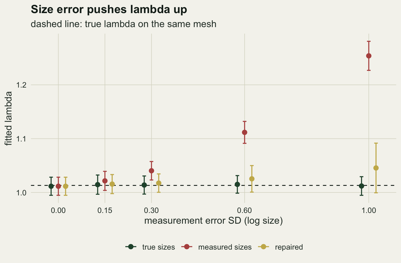
Where the bias enters
Refit with the error in one vital rate at a time and true sizes everywhere else. Growth is the one regression where size is on both sides, so it is split further: error in this year’s size only, which flattens the slope, and error in next year’s size only, which leaves the slope alone and widens the kernel.
comp_names <- c("survival", "growth", "growth_z", "growth_zp", "fecundity", "recruits", "measured")
comp6 <- sapply(comp_names, function(k) paired(main_runs[["0.6"]], k))
comp3 <- sapply(comp_names, function(k) paired(main_runs[["0.3"]], k))
sum_parts6 <- sum(comp6["bias", c("survival", "growth", "fecundity", "recruits")])
share_growth6 <- comp6["bias", "growth"] / comp6["bias", "measured"]
max_mcse6 <- max(comp6["mcse", ])
parts4 <- c("survival", "growth", "fecundity", "recruits")
lo6 <- sapply(parts4, function(k) removed(main_runs[["0.6"]], k))
At an error SD of 0.6 the full bias, measured against the fit on true sizes from the same studies, is 0.0966. Error in the growth regression alone gives 0.0645, which is 67 per cent of it. Survival alone gives 0.0113, flowering and recruit number together 0.0112, and recruit size 0.0102. The four add up to 0.0972, so in this model the parts combine almost additively. The largest Monte Carlo standard error of these paired differences is 0.0010. The other direction gives a similar split: keeping the error everywhere and refitting one rate on true sizes takes away 0.0138 for survival, 0.0631 for growth, 0.0090 for flowering and recruit number and 0.0096 for recruit size, together 0.0955 (largest Monte Carlo standard error 0.0007).
Inside the growth regression, error in this year’s size alone gives 0.0366 and error in next year’s size alone 0.0305. The second is the case the regression dilution post calls harmless for the slope, and for the slope it is. For an IPM the residual SD is a parameter of the kernel, and a wider growth density sends more plants from the middle of the size range into the large sizes where flowering and recruit numbers climb steeply. At an error SD of 0.3 the same split gives 0.0100 and 0.0086, out of a total of 0.0265.
set.seed(719)
d_one <- sim_plants(n_plants)
zo_one  <- d_one$z  + rnorm(length(d_one$z), 0, 0.6)
z1o_one <- d_one$z1 + rnorm(length(d_one$z), 0, 0.6)
alive_one <- d_one$s == 1
g_one <- fit_grow(zo_one, z1o_one, alive_one)
pts <- data.frame(z = zo_one[alive_one], zp = z1o_one[alive_one])
lines_df <- data.frame(fit = factor(c("true", "fitted to measured sizes"),
                                    levels = c("true", "fitted to measured sizes")),
                       a = c(pars[["a_g"]], g_one[1]), b = c(pars[["b_g"]], g_one[2]))
p_scatter <- ggplot(pts, aes(z, zp)) +
  geom_point(colour = te_body, alpha = 0.15, size = 0.6) +
  geom_abline(data = lines_df, aes(intercept = a, slope = b, colour = fit), linewidth = 1) +
  scale_colour_manual(values = c(te_forest, te_rust), name = NULL) +
  labs(x = "measured size this year", y = "measured size next year",
       title = "Flatter line", subtitle = "survivors, error SD 0.6") +
  theme_datasheet() + theme(legend.position = "bottom")
z_small <- 3
zp_grid <- seq(-1, 9, length.out = 400)
dens_df <- rbind(
  data.frame(zp = zp_grid, fit = "true",
             dens = dnorm(zp_grid, pars[["a_g"]] + pars[["b_g"]] * z_small, pars[["sg"]])),
  data.frame(zp = zp_grid, fit = "fitted to measured sizes",
             dens = dnorm(zp_grid, g_one[1] + g_one[2] * z_small, g_one[3])))
dens_df$fit <- factor(dens_df$fit, levels = c("true", "fitted to measured sizes"))
p_dens <- ggplot(dens_df, aes(zp, dens, colour = fit)) +
  geom_line(linewidth = 1) +
  scale_colour_manual(values = c(te_forest, te_rust), name = NULL) +
  labs(x = "size next year", y = "growth density",
       title = "Wider and shifted", subtitle = "a plant of true size 3") +
  theme_datasheet() + theme(legend.position = "bottom")
p_scatter + p_dens + plot_annotation(theme = theme_datasheet())
p_above6 <- c(true = 1 - pnorm(6, pars[["a_g"]] + pars[["b_g"]] * z_small, pars[["sg"]]),
              fitted = 1 - pnorm(6, g_one[1] + g_one[2] * z_small, g_one[3]))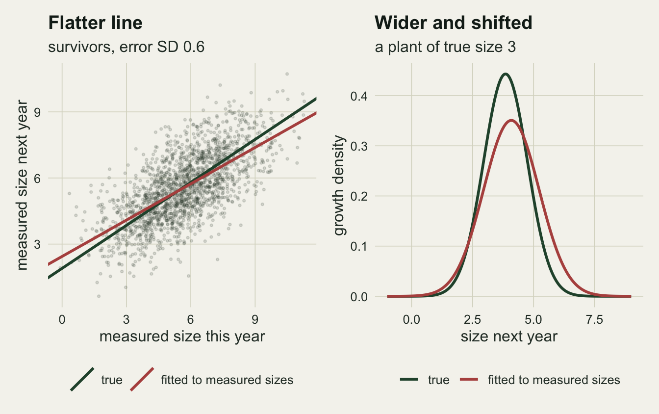
In that one study the fitted line has slope 0.549 and growth SD 1.138. For a plant of size 3 the chance of reaching size 6 or more next year is 0.008 under the true parameters and 0.046 under the measured fit. The flatter line raises the expected size of small plants and the wider density does the rest.
Steep size-dependent survival
The split above belongs to one set of vital rates. Survival in this plant rises gently with size. To see whether growth still carries most of the bias when survival rises steeply, the survival slope is tripled to 1.5 and the intercept moved to -6.6, so survival at the mean size 5.2 is unchanged. Nothing else changes, and the parameters were set before this run. The change also turns a slowly growing population into a declining one, and the comparison does not separate the two.
pars_tree <- pars; pars_tree[c("a_s", "b_s")] <- c(-6.6, 1.5)
lambda_tree <- lambda_ipm(pars_tree)
set.seed(1508)
tree_runs <- t(replicate(n_rep, one_study(0.6, p = pars_tree)))
comp_tree <- sapply(comp_names, function(k) paired(tree_runs, k))
sum_parts_tree <- sum(comp_tree["bias", c("survival", "growth", "fecundity", "recruits")])
tree_rep <- paired(tree_runs, "repaired")
lo_tree <- sapply(parts4, function(k) removed(tree_runs, k))
gr_minus_rc <- tree_runs[, "growth"] - tree_runs[, "recruits"]
gr_rc_diff <- c(mean(gr_minus_rc), sd(gr_minus_rc) / sqrt(n_rep))
gr_minus_rc_lo <- tree_runs[, "lo_recruits"] - tree_runs[, "lo_growth"]
gr_rc_diff_lo <- c(mean(gr_minus_rc_lo), sd(gr_minus_rc_lo) / sqrt(n_rep))
The steep-survival plant has a true lambda of 0.850. At an error SD of 0.6 the full bias is 0.0572. Growth alone gives 0.0185 and recruit size alone 0.0177; survival alone gives 0.0007 and flowering and recruit number alone 0.0005. Here the single-rate parts add to only 0.0375, well short of the full bias, so the errors interact rather than add. Growth and recruit size are the two largest single parts, 32 and 31 per cent of the full bias; their paired difference is 0.0008 with a Monte Carlo standard error of 0.0007, so they are level within Monte Carlo error, and neither dominates the total.
Taken the other way round, with the error kept everywhere and one rate refitted on true sizes, removing the survival error takes away 0.0154 of the bias, growth 0.0366, recruit size 0.0227 and flowering and recruit number 0.0006 (largest Monte Carlo standard error 0.0008). These four add to 0.0752, more than the full bias, where the error-in-one-rate parts added to less. In this direction growth and recruit size are not level: removing the growth error takes away 0.0139 more than removing the recruit-size error (Monte Carlo standard error 0.0007). Survival error on its own adds almost nothing, yet removing it takes away 27 per cent of the full bias: here survival error acts through its interaction with the error in the other rates, and since flowering and recruit number carry almost none in either direction, that means growth, recruit size or both. Neither direction gives a unique share per rate. What transfers from the first plant is the sign, not the split.
comp_labels <- c(survival = "survival", growth = "growth (both sizes)",
                 growth_z = "growth, this year's size", growth_zp = "growth, next year's size",
                 fecundity = "flowering and recruit number", recruits = "recruit size",
                 measured = "all sizes")
comp_df <- rbind(
  data.frame(model = "gentle survival (slope 0.5)", part = comp_names,
             bias = comp6["bias", ], mcse = comp6["mcse", ]),
  data.frame(model = "steep survival (slope 1.5)", part = comp_names,
             bias = comp_tree["bias", ], mcse = comp_tree["mcse", ]))
comp_df$part <- factor(comp_labels[comp_df$part], levels = rev(comp_labels))
comp_df$kind <- ifelse(comp_df$part == "all sizes", "all", "one rate")
ggplot(comp_df, aes(bias, part, colour = kind)) +
  geom_vline(xintercept = 0, colour = te_ink, linewidth = 0.4) +
  geom_errorbar(aes(xmin = bias - 2 * mcse, xmax = bias + 2 * mcse),
                orientation = "y", width = 0.3, linewidth = 0.6) +
  geom_point(size = 2.6) +
  scale_colour_manual(values = c(all = te_rust, `one rate` = te_forest), guide = "none") +
  facet_wrap(~model) +
  scale_x_continuous(breaks = c(0, 0.03, 0.06, 0.09)) +
  labs(x = "bias in lambda (measured minus true sizes)", y = NULL,
       title = "Where the bias enters",
       subtitle = "error SD 0.6, error confined to one vital rate at a time") +
  theme_datasheet() + theme(strip.text = element_text(colour = te_ink, face = "bold"),
                            panel.spacing = unit(1.5, "lines"))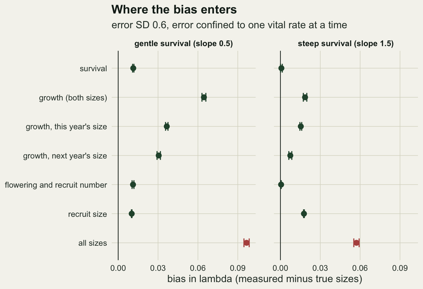
More plants do not help
The bias from measurement error does not shrink as more plants are marked. Sampling noise does, so the ratio of the two grows with the size of the study.
set.seed(3008)
n_grid <- c(300, 1000)
ns_rows <- lapply(n_grid, function(nn) lapply(c(0.3, 0.6), function(se) {
  r <- t(replicate(n_rep, one_study(se, n = nn, extras = FALSE)))
  data.frame(n = nn, se = se, bias = mean(r[, "measured"]) - lambda_true,
             sd = sd(r[, "measured"]), bias_exact = mean(r[, "exact"]) - lambda_true)
}))
ns <- do.call(rbind, unlist(ns_rows, recursive = FALSE))
ns <- rbind(ns, data.frame(n = n_plants, se = c(0.3, 0.6),
                           bias = c(at_se("meas", 0.3), at_se("meas", 0.6)) - lambda_true,
                           sd = c(at_se("sd_meas", 0.3), at_se("sd_meas", 0.6)),
                           bias_exact = c(at_se("exact", 0.3), at_se("exact", 0.6)) - lambda_true))
ns$bias_net <- ns$bias - ns$bias_exact
ns$ratio <- ns$bias / ns$sd
ns_at <- function(col, nn, se) ns[[col]][ns$n == nn & ns$se == se]
With 300 plants and an error SD of 0.3 the bias against the true lambda is 0.038 with an across-study SD of 0.059, a ratio of 0.65; the ratio is 0.68 with 1000 plants and 1.59 with 2600, below two SDs at every size tried. The flat stretch between 300 and 1000 plants is Monte Carlo noise in the true-size reference: the fit on true sizes itself sits 0.011 above the true lambda at 300 plants and 0.004 below it at 1000, and the figure, which measures bias against the true lambda, carries that noise. Measured instead against the fit on true sizes from the same studies, the bias at an error SD of 0.3 is 0.027, 0.026 and 0.027 at the three sizes, and at 0.6 it is 0.095, 0.099 and 0.097. At 0.6 the ratio to the across-study SD is 1.55 with 300 plants, 2.94 with 1000 and 4.83 with 2600. A large, carefully fitted census gives a narrow interval around the wrong value.
A two-number repair
The repair needs one extra piece of field work: measure a random subsample of plants twice, independently, in the same census. Half the variance of the differences estimates the error variance. With that one number, and the variance of measured size, three corrections follow.
For survival, flowering and recruit number, each measured size is replaced by its expected true size given the measurement, which under normal sizes shrinks it towards the mean by the reliability ratio (regression calibration; Carroll et al. 2006). For growth, the slope is the covariance of the two measured sizes divided by the variance of measured size minus the error variance, and the growth variance is the residual variance with both error contributions subtracted. For recruit size, the error variance comes off the observed variance. Here the subsample is 100 plants, fixed in the design chunk.
The growth part is the method of moments for a linear model with a latent size. A marginal likelihood that treats true size as a normal latent variable, with the error variance fixed, has five parameters for five sample moments and returns the same answer, which the next chunk checks on one study.
alive_ch <- alive_one
v_err_one <- 0.6^2
xm <- zo_one[alive_ch]; ym <- z1o_one[alive_ch]
nll_latent <- function(th) {
  mu <- th[1]; tau2 <- exp(th[2]); a <- th[3]; b <- th[4]; s2 <- exp(th[5])
  S <- matrix(c(tau2 + v_err_one, b * tau2, b * tau2, b^2 * tau2 + s2 + v_err_one), 2)
  r <- cbind(xm - mu, ym - a - b * mu)
  Si <- solve(S)
  0.5 * (length(xm) * log(det(S)) + sum((r %*% Si) * r))
}
opt <- optim(c(mean(xm), log(var(xm)), 2, 0.6, log(0.8)), nll_latent,
             method = "BFGS", control = list(maxit = 500, reltol = 1e-12))
vx <- mean((xm - mean(xm))^2); vy <- mean((ym - mean(ym))^2)
cxy <- mean((xm - mean(xm)) * (ym - mean(ym)))
b_mom <- cxy / (vx - v_err_one)
s_mom <- sqrt(vy - v_err_one - b_mom^2 * (vx - v_err_one))
latent_gap <- max(abs(c(opt$par[4] - b_mom, sqrt(exp(opt$par[5])) - s_mom)))
On the study drawn for the figure, with the error variance set to its true value, the latent-size likelihood gives a growth slope of 0.614 and the moment formula 0.614; the two estimates of slope and growth SD differ by at most 2.0e-06. For Gaussian growth and Gaussian error nothing is gained from the likelihood. It earns its keep once growth is not linear or error is not normal, and in state-space IPMs fitted to survey time series where individuals are not followed (White et al. 2016).
rep6 <- paired(main_runs[["0.6"]], "repaired")
rep3 <- paired(main_runs[["0.3"]], "repaired")
rep10 <- paired(main_runs[["1"]], "repaired")
rep_ratio <- function(se) (at_se("rep", se) - lambda_true) / at_se("sd_rep", se)
Back in the hundred studies per error level, the repaired lambda averages 1.017 at an error SD of 0.3, 1.025 at 0.6 and 1.046 at 1.0. Its remaining bias against the fit on true sizes is 0.0036, 0.0103 and 0.0335 (Monte Carlo standard errors 0.0006, 0.0018 and 0.0041). Measured against the true lambda, the remaining bias is 0.50 across-study SDs at 0.6 and 0.70 at 1.0, down from 4.8 and 8.9. It is not free. The across-study SD of the repaired lambda is 0.025 at 0.6 and 0.046 at 1.0, against 0.020 and 0.027 without it: the correction divides by an error variance estimated from 100 pairs. In the steep-survival plant the repair leaves a bias of -0.0048 (Monte Carlo standard error 0.0011), a slight overcorrection, where the uncorrected bias was 0.0572.
ns$error <- factor(sprintf("error SD %.1f", ns$se))
ggplot(ns, aes(n, ratio, colour = error)) +
  geom_hline(yintercept = c(0, 2), linetype = c("solid", "dashed"), colour = te_ink,
             linewidth = 0.4) +
  geom_line(linewidth = 0.9) + geom_point(size = 2.4) +
  scale_x_log10(breaks = c(300, 1000, 2600)) +
  scale_colour_manual(values = c(te_gold, te_rust), name = NULL) +
  labs(x = "marked plants (log scale)", y = "bias / across-study SD",
       title = "The bias outgrows the noise",
       subtitle = "dashed line: two SDs") +
  theme_datasheet() + theme(legend.position = "bottom")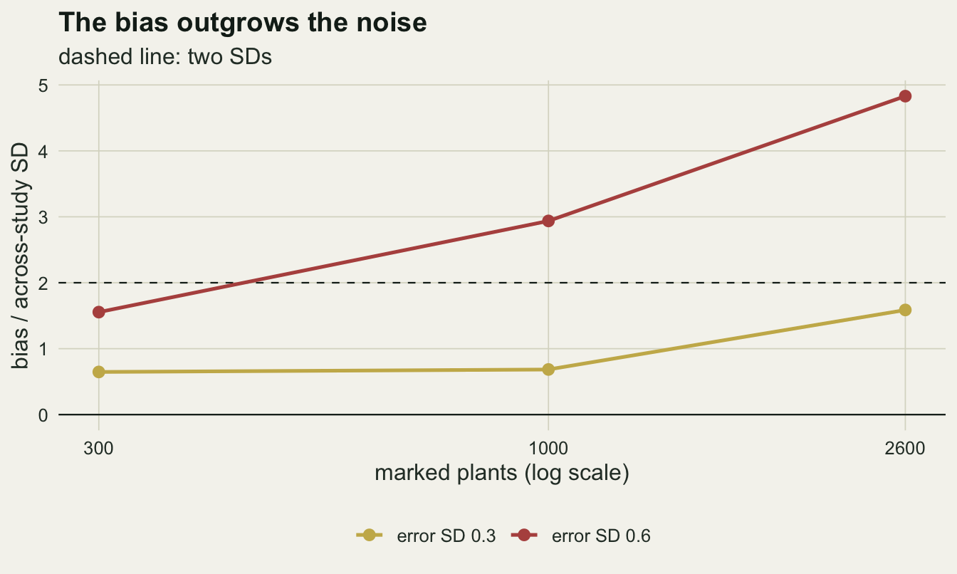
The shrinker rule
A common cleaning step removes survivors recorded as smaller next year, on the grounds that the plant cannot really have shrunk. In this plant it can: growth regresses towards an equilibrium size, and large plants shrink.
shr <- vapply(main_runs, function(r) c(meas = mean(r[, "shrink_meas"]),
                                        true = mean(r[, "shrink_true"]),
                                        lam = mean(r[, "no_shrinkers"])), numeric(3))
Without any measurement error 52 per cent of survivors shrink, and dropping them gives a lambda of 1.299. At an error SD of 0.6 the recorded share is 52 per cent and the rule gives 1.429. The rule removes the plants that hold the kernel near equilibrium, and it does so whether or not the data carry error. A species in which true shrinkage is rare was not simulated; there the rule removes plants whose second measurement fell below the first by chance, which raises the fitted mean growth and narrows its spread, with a net effect on lambda that was not measured. In the simulation the rule drops those plants from the growth regression only; survival, flowering and recruit number keep them.
What to report
Give the measurement protocol for size and a number for its repeatability. An error SD of 0.3 on log size moved lambda from 1.013 to 1.040 here, and a reader cannot guess from “leaf length was measured” whether that applies.
Remeasure a random subsample in at least one census, blind to the first measurement, and report the estimated error variance with the number of pairs. A same-census remeasurement by one person misses any between-observer part of the error, so the subsample should be remeasured by the census observers. With 100 pairs the repair took the bias at an error SD of 0.6 from 4.8 across-study SDs to 0.50.
Report lambda with and without the correction. If the two differ by more than the interval width, the growth rate is a statement about the measurement protocol as much as about the population.
Do not delete shrinkers from the growth regression. Setting negative growth to zero was not simulated here. Model the error instead.
Honest limits
Error here is classical, normal, constant across sizes and independent between the two censuses. If the error is a fixed number of millimetres rather than a fixed fraction, its SD on log size is larger for small plants, which are where Louthan and Doak locate the effect; the constant-variance correction above does not allow for that. An observer who carries a personal bias from one census to the next makes errors that are correlated across years, and those partly cancel in the growth increment. Neither case was simulated.
No field estimate of error SD is used. An error SD of 0.6, where most headline numbers above sit, means a typical measurement is off by a factor of 1.82: plausible for scored cover or visually estimated biomass, and large for a measured leaf or stem. At 0.15, a factor of 1.16, lambda from the measured sizes is 1.022 against the true 1.013, a bias of 0.5 across-study SDs. The grid from 0.15 to 1.0 is a sensitivity range, not a summary of published error rates, and the right value for a given species and protocol has to come from a remeasurement, which is the point of the repair.
Regression calibration for logistic and Poisson regressions is an approximation that assumes normal true sizes. The size distribution here is a truncated normal, and flowering plants are a size-biased subset. The approximation is one candidate for the residual bias of 0.0335 at the largest error level; the sources of that residual were not separated. SIMEX or a latent-size likelihood for all four rates are the next steps, and neither was run.
The year-to-year link is simplified. Each simulated study has one transition with independent sizes; in a real census next year’s measured size is also next year’s predictor, and recruits enter the next size measurement. Louthan and Doak also simulated temporal and individual-based error types; neither is present here.
The component split was measured for two parameter sets. The additive split in the first and the interaction in the second (with its dependence on the order in which rates are reset) are both results for those parameters, not general rules.
References
Louthan AM, Doak DF 2018 Ecology 99(10):2308-2317 (10.1002/ecy.2455)
Easterling MR, Ellner SP, Dixon PM 2000 Ecology 81(3):694-708 (10.1890/0012-9658(2000)081[0694:SSSAAN]2.0.CO;2)
White JW, Nickols KJ, Malone D, Carr MH, Starr RM, Cordoleani F, Baskett ML, Hastings A, Botsford LW 2016 Ecological Applications 26(8):2677-2694 (10.1002/eap.1398)
Carroll RJ, Ruppert D, Stefanski LA, Crainiceanu CM 2006 Measurement Error in Nonlinear Models: A Modern Perspective, 2nd edition (ISBN 9781584886334)