library(ggplot2)

te_paper  <- "#f5f4ee"
te_ink    <- "#16241d"
te_body   <- "#2c3a31"
te_forest <- "#275139"
te_rust   <- "#b5534e"
te_gold   <- "#c9b458"
te_line   <- "#dad9ca"

theme_datasheet <- function() {
  theme_minimal(base_size = 12) +
    theme(plot.background  = element_rect(fill = te_paper, colour = NA),
          panel.background = element_rect(fill = te_paper, colour = NA),
          panel.grid.major = element_line(colour = te_line, linewidth = 0.3),
          panel.grid.minor = element_blank(),
          text             = element_text(colour = te_body),
          plot.title       = element_text(colour = te_ink, face = "bold"),
          plot.subtitle    = element_text(colour = te_body),
          axis.text        = element_text(colour = te_body))
}Siblings in an assignment baseline
R
population genetics
simulation
ecology tutorial
ggplot2
Full-sib families in an assignment baseline make the exclusion test reject genuine residents. In R: how often, why, and a null that simulates the family design.
A fisheries team wants to know which river each young salmon in a coastal mixture came from. The baseline is 40 genotyped juveniles per river, and the juveniles were caught the cheap way: a few electrofishing passes at one or two spawning riffles in each river, in late summer. Parr from one riffle are not a random sample of the river’s gene pool. They are a handful of families, and five or ten fish from the same pair of parents are common. The same happens with glass eels caught on one night, with hatchlings from a few turtle nests and with seed lots from a few mother trees.
Assignment tests and self-assignment builds the machinery used below: a genotype likelihood from estimated allele frequencies, a leave-one-out correction for self-assignment, and an exclusion test that asks whether a genotype is the kind that a source produces at all, which that post calls “the single check that separates a defensible assignment from a confident guess”. Its honest limits name the family problem and stop there: “A baseline of 40 that contains sibling groups carries fewer independent gene copies than 80, so the estimated frequencies are pulled towards a few families, the source looks tighter than it is, and both the self-assignment rate and the exclusion test become optimistic. The leave-one-out correction removes one individual, not its siblings.” This post measures both halves of that sentence with the same code, and leads with the exclusion test, because the failure there is the one that decides whether a fish is reported as coming from an unsampled river.
The self-assignment half is not new. Ostergren and colleagues showed in 2020, for Atlantic salmon baselines, that self-assignment accuracy rises as family structure in the baseline increases while the accuracy on fish of known origin falls; it is demonstrated here with the source post’s own code, and credited to them. The exclusion test was not part of their study. Two other posts on this site touch the neighbourhood. Data leakage in ecological model validation shows that random folds leak when rows share a site, and that leaving one site out “tracks the error on sites the model has never seen”; leaving a family out of an assignment baseline turns out to behave differently when families are few. Purging siblings before estimating Ne deals with samples built from families for effective size, not for assignment.
A baseline built from families
The first five functions below are copied from the source post without change: the genotype log-likelihood (with its heterozygote term), the frequency estimate with half a count added to each allele, the Balding-Nichols frequencies around an ancestral value, Hardy-Weinberg genotypes, and the leave-one-out scoring. The family generator is new. It draws two Hardy-Weinberg parents per family, and each offspring receives one allele from each parent at every locus, with loci unlinked.
geno_loglik <- function(geno, p) {
  as.vector(geno %*% log(p) + (2 - geno) %*% log(1 - p)) +
    rowSums(geno == 1) * log(2)
}

est_freq <- function(geno, k = 0.5) {
  (colSums(geno) + k) / (2 * nrow(geno) + 2 * k)
}

sim_freqs <- function(n_loci, n_src, fst) {
  p_anc <- runif(n_loci, 0.05, 0.95)
  shape_a <- p_anc * (1 - fst) / fst
  shape_b <- (1 - p_anc) * (1 - fst) / fst
  matrix(rbeta(n_loci * n_src, rep(shape_a, n_src), rep(shape_b, n_src)),
         n_loci, n_src)
}

sim_geno <- function(p, n_ind) {
  matrix(rbinom(n_ind * length(p), 2, rep(p, each = n_ind)), n_ind, length(p))
}

loo_loglik <- function(ll, geno_list, who, k = 0.5) {
  for (s in seq_along(geno_list)) {
    g_s <- geno_list[[s]]
    tot <- colSums(g_s)
    rows <- which(who == s)
    for (q in seq_along(rows)) {
      p_out <- (tot - g_s[q, ] + k) / (2 * (nrow(g_s) - 1) + 2 * k)
      ll[rows[q], s] <- geno_loglik(g_s[q, , drop = FALSE], p_out)
    }
  }
  ll
}

# new: n_fam full-sib families of fam_size offspring (fam_size = 1 gives unrelated fish)
sim_families <- function(p, n_fam, fam_size) {
  if (fam_size == 1) return(list(geno = sim_geno(p, n_fam), fam = seq_len(n_fam)))
  n_l <- length(p)
  mum <- sim_geno(p, n_fam); dad <- sim_geno(p, n_fam)
  fam_id <- rep(seq_len(n_fam), each = fam_size)
  n_off <- n_fam * fam_size
  geno <- matrix(rbinom(n_off * n_l, 1, as.vector(mum[fam_id, ] / 2)), n_off) +
    matrix(rbinom(n_off * n_l, 1, as.vector(dad[fam_id, ] / 2)), n_off)
  list(geno = geno, fam = fam_id)
}
The design follows the source post’s self-assignment section: three sources at a target Fst of 0.03, 100 biallelic loci, 40 baseline fish per source. The 40 fish come as 40 unrelated individuals, as 20 families of 2, as 8 families of 5 or as 4 families of 10.
How much a family baseline is worth has a short closed form. Two full sibs have a kinship coefficient of a quarter: a gene copy drawn from each is identical by descent with probability 1/4. Each fish carries two copies, so the covariance of their allele counts at a locus is \(4 \times \tfrac14\,pq = pq\), against a variance of \(2pq\) for one fish. A family of \(S\) sibs then contributes a variance of \(pq\,S(S+1)\) to the allele total, and the frequency estimated from \(F\) such families has variance \(pq\,(S+1)/(4FS)\). Writing that as \(pq/m\) gives the number of independent gene copies the baseline is worth, \(m = 4FS/(S+1)\), against \(2FS\) copies on paper.
n_loci <- 100; n_src <- 3; fst_target <- 0.03; n_ind <- 40
designs <- data.frame(name = c("40 unrelated", "20 x 2", "8 x 5", "4 x 10"),
                      n_fam = c(40, 20, 8, 4), fam_size = c(1, 2, 5, 10))
designs$m_eff <- 4 * designs$n_fam * designs$fam_size / (designs$fam_size + 1)

set.seed(56001)
p_check <- runif(n_loci, 0.1, 0.9)
m_sim <- sapply(seq_len(nrow(designs)), function(d) {
  raw <- replicate(600, colSums(sim_families(p_check, designs$n_fam[d],
                                             designs$fam_size[d])$geno)) / (2 * n_ind)
  mean(p_check * (1 - p_check) / apply(raw, 1, var))
})
designs$m_sim <- m_sim
print(designs, row.names = FALSE, digits = 3)
name n_fam fam_size m_eff m_sim
40 unrelated 40 1 80.0 81.0
20 x 2 20 2 53.3 53.7
8 x 5 8 5 26.7 26.7
4 x 10 4 10 14.5 14.6Over 600 simulated baselines per design, the effective number of gene copies measured from the spread of the raw allele proportions is 81.0, 53.7, 26.7 and 14.6, against 80.0, 53.3, 26.7 and 14.5 from the formula. Eight families of five are worth about as much as 13 unrelated fish, and four families of ten about as much as 7. That is arithmetic, and the rest of the post is about what the arithmetic does to two procedures that count 80 copies.
Three nulls for the exclusion test
The source post’s exclusion test draws null genotypes from the source and asks how often they score at or below the fish in question. Its null frequencies are drawn from a beta posterior on 80 gene copies, the same half-count correction as the estimate, and every null genotype is scored against the estimated frequencies. Locating a genotype in a simulated distribution of genotypes from the candidate source is the exclusion idea of Cornuet and colleagues (1999). A genuine resident, a fish of that source that was not in the baseline, should be excluded at the nominal rate of 0.05.
Two alternatives are compared with it. The first keeps the source post’s null but counts the gene copies correctly, drawing the null frequencies from a beta posterior on \(m\) copies instead of \(2FS\). The second simulates the whole baseline step: draw a new baseline of the same \(F\) families of \(S\) from the estimated frequencies, re-estimate frequencies from it, and score a new genotype drawn at the estimated frequencies against the re-estimate. That is a parametric bootstrap of the estimation, and it needs \(F\) and \(S\). The allele total of a simulated family baseline does not need individual fish: each parent is homozygous for the counted allele, heterozygous or neither, a homozygous parent passes the allele to all \(S\) offspring and a heterozygous parent to a binomial number of them, so the total is drawn from three binomials.
n_fresh <- 100; n_null <- 3000; alpha <- 0.05

null_post <- function(geno, copies = 2 * nrow(geno)) {
  n <- nrow(geno); raw <- colSums(geno) / (2 * n); ph <- est_freq(geno)
  p_star <- matrix(rbeta(n_null * n_loci, rep(raw * copies + 0.5, each = n_null),
                         rep((1 - raw) * copies + 0.5, each = n_null)), n_null, n_loci)
  sort(geno_loglik(matrix(rbinom(n_null * n_loci, 2, as.vector(p_star)), n_null, n_loci), ph))
}

null_from <- function(p_gen, n_fam, fam_size) {  # simulate the baseline step from p_gen (vector, or one row per null fish)
  php <- if (is.matrix(p_gen)) as.vector(p_gen) else rep(p_gen, each = n_null)
  if (fam_size == 1) {
    tot <- rbinom(n_null * n_loci, 2 * n_fam, php)
  } else {
    n_hom <- rbinom(n_null * n_loci, 2 * n_fam, php^2)
    n_het <- rbinom(n_null * n_loci, 2 * n_fam - n_hom, 2 * php * (1 - php) / (1 - php^2))
    tot <- fam_size * n_hom + rbinom(n_null * n_loci, fam_size * n_het, 0.5)
  }
  p_re <- matrix((tot + 0.5) / (2 * n_fam * fam_size + 1), n_null, n_loci)
  g_new <- matrix(rbinom(n_null * n_loci, 2, php), n_null, n_loci)
  sort(rowSums(g_new * log(p_re) + (2 - g_new) * log(1 - p_re)) + rowSums(g_new == 1) * log(2))
}
null_design <- function(geno, n_fam, fam_size) null_from(est_freq(geno), n_fam, fam_size)

p_value <- function(null_sorted, obs) findInterval(obs, null_sorted) / length(null_sorted)
With copies left at its default of \(2n\), the beta shapes are the allele count plus a half and the complement plus a half, exactly as in the source post, and its 3000 null genotypes are kept.
self_rates <- function(bl) {
  gl <- lapply(bl, `[[`, "geno"); fl <- lapply(bl, `[[`, "fam")
  who <- rep(seq_along(gl), sapply(gl, nrow)); g_all <- do.call(rbind, gl)
  ph <- sapply(gl, est_freq)
  ll_in <- sapply(seq_along(gl), function(s) geno_loglik(g_all, ph[, s]))
  hit <- function(ll, w) mean(apply(ll, 1, which.max) == w)
  ll_lfo <- ll_in                                  # leave the whole family out
  for (s in seq_along(gl)) {
    tot <- colSums(gl[[s]]); rows <- which(who == s)
    for (f in unique(fl[[s]])) {
      in_f <- which(fl[[s]] == f)
      p_out <- (tot - colSums(gl[[s]][in_f, , drop = FALSE]) + 0.5) /
        (2 * (nrow(gl[[s]]) - length(in_f)) + 1)
      ll_lfo[rows[in_f], s] <- geno_loglik(gl[[s]][in_f, , drop = FALSE], p_out)
    }
  }
  gp <- lapply(seq_along(gl), function(s) gl[[s]][!duplicated(fl[[s]]), , drop = FALSE])
  who_p <- rep(seq_along(gp), sapply(gp, nrow)); g_p <- do.call(rbind, gp)
  ll_p <- sapply(seq_along(gp), function(s) geno_loglik(g_p, est_freq(gp[[s]])))
  c(naive = hit(ll_in, who), loo = hit(loo_loglik(ll_in, gl, who), who),
    lfo = hit(ll_lfo, who), purge = hit(loo_loglik(ll_p, gp, who_p), who_p))
}

score_design <- function(p_set, fresh, n_fam, fam_size, wide = TRUE, mis = FALSE) {
  bl <- lapply(1:n_src, function(s) sim_families(p_set[, s], n_fam, fam_size))
  ph <- sapply(bl, function(b) est_freq(b$geno))
  m_copies <- 4 * n_fam * fam_size / (fam_size + 1)
  g_fresh <- do.call(rbind, fresh[1:n_src]); who_f <- rep(1:n_src, sapply(fresh[1:n_src], nrow))
  ll_f <- sapply(1:n_src, function(s) geno_loglik(g_fresh, ph[, s]))
  res <- c(size_post = 0, size_wide = NA, size_des = 0, size_as_4x10 = NA,
           size_as_20x2 = NA, size_as_unrel = NA, ll_obs = 0, ll_truth = 0,
           ll_post = 0, ll_des = 0, sd_post = 0, sd_des = 0)
  if (wide && fam_size > 1) res["size_wide"] <- 0
  if (mis) res[c("size_as_4x10", "size_as_20x2", "size_as_unrel")] <- 0
  out_post <- out_des <- out_4x10 <- out_20x2 <- out_unrel <- matrix(FALSE, nrow(fresh[[4]]), n_src)
  res_post <- res_des <- matrix(FALSE, nrow(g_fresh), n_src)   # residents of all sources vs each null
  for (s in 1:n_src) {
    g <- bl[[s]]$geno
    obs <- geno_loglik(fresh[[s]], ph[, s]); o4 <- geno_loglik(fresh[[4]], ph[, s])
    np <- null_post(g); nd <- null_design(g, n_fam, fam_size)
    res["size_post"] <- res["size_post"] + mean(p_value(np, obs) < alpha) / n_src
    res["size_des"] <- res["size_des"] + mean(p_value(nd, obs) < alpha) / n_src
    if (!is.na(res["size_wide"])) res["size_wide"] <- res["size_wide"] +
      mean(p_value(null_post(g, m_copies), obs) < alpha) / n_src
    if (mis) {
      n_4x10 <- null_design(g, 4, 10); n_20x2 <- null_design(g, 20, 2)
      res["size_as_4x10"] <- res["size_as_4x10"] + mean(p_value(n_4x10, obs) < alpha) / n_src
      res["size_as_20x2"] <- res["size_as_20x2"] + mean(p_value(n_20x2, obs) < alpha) / n_src
      n_unrel <- null_design(g, 40, 1)
      res["size_as_unrel"] <- res["size_as_unrel"] + mean(p_value(n_unrel, obs) < alpha) / n_src
      out_4x10[, s] <- p_value(n_4x10, o4) < alpha; out_20x2[, s] <- p_value(n_20x2, o4) < alpha
      out_unrel[, s] <- p_value(n_unrel, o4) < alpha
    }
    res[c("ll_obs", "ll_truth", "ll_post", "ll_des", "sd_post", "sd_des")] <-
      res[c("ll_obs", "ll_truth", "ll_post", "ll_des", "sd_post", "sd_des")] +
      c(mean(obs), mean(geno_loglik(fresh[[s]], p_set[, s])), mean(np), mean(nd), sd(np), sd(nd)) / n_src
    out_post[, s] <- p_value(np, o4) < alpha; out_des[, s] <- p_value(nd, o4) < alpha
    res_post[, s] <- p_value(np, ll_f[, s]) < alpha; res_des[, s] <- p_value(nd, ll_f[, s]) < alpha
  }
  sr <- self_rates(bl)
  if (fam_size == 1) sr[c("lfo", "purge")] <- NA
  pw_mis <- if (mis) c(power_as_4x10 = mean(rowSums(out_4x10) == n_src),
                       power_as_20x2 = mean(rowSums(out_20x2) == n_src),
                       power_as_unrel = mean(rowSums(out_unrel) == n_src)) else
    c(power_as_4x10 = NA, power_as_20x2 = NA, power_as_unrel = NA)
  c(res, power_post = mean(rowSums(out_post) == n_src), power_des = mean(rowSums(out_des) == n_src),
    pw_mis, all3_post = mean(rowSums(res_post) == n_src), all3_des = mean(rowSums(res_des) == n_src),
    sr, truth = mean(apply(ll_f, 1, which.max) == who_f))
}

run_sets <- function(n_sets, fst, dsg, ...) {
  do.call(rbind, lapply(seq_len(n_sets), function(i) {
    p_set <- sim_freqs(n_loci, n_src + 1, fst)          # the fourth source is never sampled
    fresh <- lapply(1:(n_src + 1), function(s) sim_geno(p_set[, s], n_fresh))
    do.call(rbind, lapply(seq_len(nrow(dsg)), function(d) data.frame(
      set = i, design = dsg$name[d],
      t(score_design(p_set, fresh, dsg$n_fam[d], dsg$fam_size[d],
                     mis = dsg$fam_size[d] == 5, ...)))))
  }))
}
mean_se <- function(tab, col, dsg) {
  v <- tab[[col]][tab$design == dsg]
  c(mean = mean(v), se = sd(v) / sqrt(length(v)))
}
Each simulated set draws frequencies for four sources, builds baselines for the first three, and draws 100 fresh fish per source that were not in any baseline. The fresh fish of sources one to three are genuine residents; those of the fourth, never sampled, source are what the exclusion test exists to catch. The fresh fish are unrelated to each other and to the baseline families.
The exclusion test turns on its own residents
designs_main <- rbind(designs[, c("name", "n_fam", "fam_size")],
                      data.frame(name = c("13 unrelated", "7 unrelated"),
                                 n_fam = c(13, 7), fam_size = 1))
n_sets <- 24
set.seed(56010)
grid_main <- run_sets(n_sets, fst_target, designs_main)
ms <- function(col, dsg) mean_se(grid_main, col, dsg)
size_tab <- do.call(rbind, lapply(designs_main$name, function(nm) rbind(
  data.frame(design = nm, null = "source post's null", t(ms("size_post", nm))),
  data.frame(design = nm, null = "beta on effective copies", t(ms("size_wide", nm))),
  data.frame(design = nm, null = "whole-design null", t(ms("size_des", nm))))))
size_tab <- size_tab[!is.na(size_tab$mean), ]
sz <- function(nm, nl) size_tab$mean[size_tab$design == nm & size_tab$null == nl]
se_max <- max(size_tab$se)
per_set_85 <- grid_main$size_post[grid_main$design == "8 x 5"]
With 40 unrelated fish per source, the source post’s null excludes 0.081 of genuine fresh residents from their own source (Monte Carlo standard error 0.004, over 24 sets of frequencies). With 20 families of 2 the rate is 0.117, with 8 families of 5 it is 0.273, and with 4 families of 10 it is 0.639. At 8 families of 5 the rate lies between 0.210 and 0.383 across the individual sets, so no draw of frequencies rescues it. The test is meant to wrongly exclude one resident in twenty. With four families of ten per source it wrongly excludes 64 in a hundred from their own source, and 56 in a hundred are excluded from all three baselines, that is, reported as having no plausible source in the baseline. The whole-design null does that to 8 in a hundred.
The two unrelated baselines at the bottom of the figure below carry roughly the effective copies of the two larger family designs. With 13 unrelated fish per source the source post’s null excludes 0.156 of residents, and with 7 unrelated fish 0.261. So the source post’s null is anti-conservative for any baseline that carries few independent gene copies, related or not, and even at 40 unrelated fish it sits above 0.05. Counting the copies correctly brings a family baseline down to about the level of the unrelated baseline it is worth: 0.149 at 8 families of 5 and 0.267 at 4 families of 10. The whole-design null gives 0.055, 0.067, 0.089 and 0.150 for the four designs of 40 fish, and 0.066 and 0.077 for the two small unrelated baselines. No Monte Carlo standard error behind the figure exceeds 0.016.
size_tab$design <- factor(size_tab$design, levels = rev(designs_main$name))
size_tab$null <- factor(size_tab$null, levels = c("source post's null", "beta on effective copies",
                                                  "whole-design null"))
p_size <- ggplot(size_tab, aes(mean, design, colour = null)) +
  geom_vline(xintercept = alpha, colour = te_body, linetype = "dashed", linewidth = 0.4) +
  geom_errorbar(aes(xmin = pmax(mean - 2 * se, 0), xmax = mean + 2 * se), orientation = "y",
                width = 0.3, linewidth = 0.4, position = position_dodge(width = 0.6)) +
  geom_point(size = 2.6, position = position_dodge(width = 0.6)) +
  scale_colour_manual(values = c(te_rust, te_gold, te_forest), name = NULL) +
  scale_x_continuous(limits = c(0, NA)) +
  labs(x = "genuine residents excluded from their own source", y = "baseline per source",
       title = "Families make the exclusion test reject residents") +
  guides(colour = guide_legend(nrow = 1)) +
  theme_datasheet() + theme(legend.position = "bottom")
p_size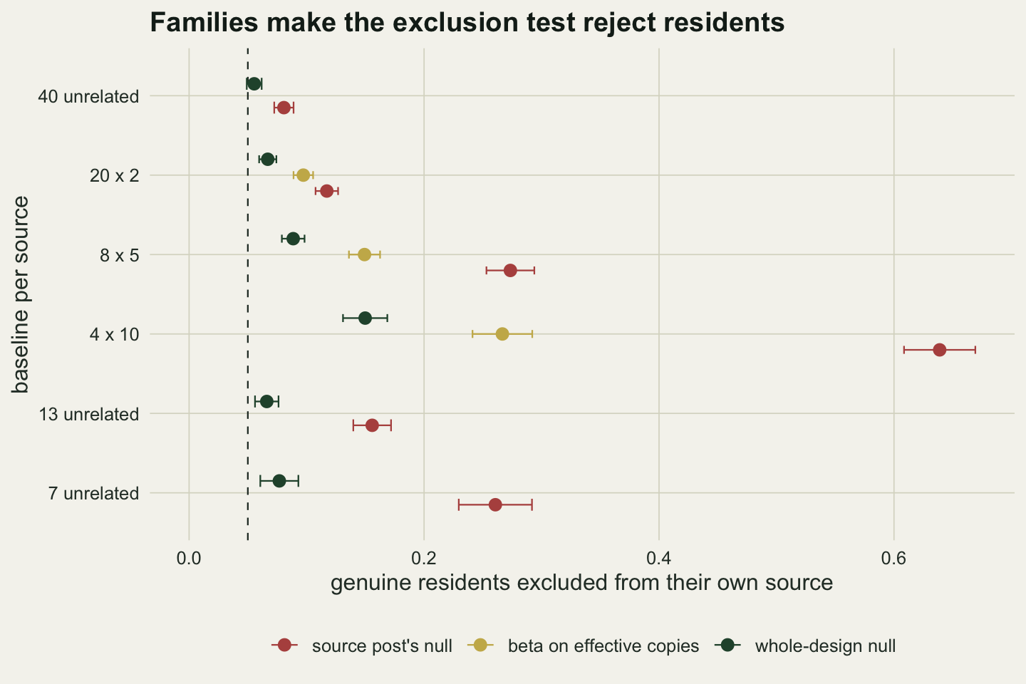
What a resident loses by being scored against an estimate
A fresh resident is scored against estimated frequencies, not the true ones, and it pays for the difference in log-likelihood. The null has to charge the same price, and the source post’s null does not: it draws genotypes around the estimate and scores them against that same estimate. The chunk below reads off the mean log-likelihoods that the grid recorded, averaged over sources and sets.
shift_tab <- do.call(rbind, lapply(designs_main$name, function(nm) {
  x <- grid_main[grid_main$design == nm, ]
  data.frame(design = nm, resident_vs_truth = mean(x$ll_truth), resident_vs_estimate = mean(x$ll_obs),
             source_null = mean(x$ll_post), design_null = mean(x$ll_des),
             gap_source_sd = mean((x$ll_post - x$ll_obs) / x$sd_post),
             gap_design_sd = mean((x$ll_des - x$ll_obs) / x$sd_des))
}))
print(shift_tab, row.names = FALSE, digits = 3)
design resident_vs_truth resident_vs_estimate source_null design_null
40 unrelated -81.1 -82.3 -81.2 -82.1
20 x 2 -81.1 -82.9 -80.8 -82.4
8 x 5 -81.1 -85.1 -79.5 -83.2
4 x 10 -81.1 -89.6 -77.0 -84.7
13 unrelated -81.1 -84.7 -81.4 -84.2
7 unrelated -81.1 -87.7 -81.9 -86.8
gap_source_sd gap_design_sd
0.204 0.0331
0.397 0.1005
1.023 0.2912
2.356 0.6377
0.602 0.0981
1.019 0.1438sh <- function(nm, col) shift_tab[[col]][shift_tab$design == nm]Scored against the true frequencies, a resident’s mean log-likelihood is about -81.1 in every design. Scored against the frequencies estimated from 40 unrelated fish it drops to -82.3, from 8 families of 5 to -85.1 and from 4 families of 10 to -89.6. The mean of the source post’s null stays near the truth-scored value or moves the other way, to -81.2, -79.5 and -77.0. It rises with families, which is what to expect when frequencies estimated from a few families are more extreme than the true ones, and a null that draws around them on 80 copies treats that spread as real, so its genotypes are more predictable than a real fish. Expressed in standard deviations of that null, the residents sit 0.20 below its mean with 40 unrelated fish, 1.02 below with 8 families of 5 and 2.36 below with 4 families of 10. A test whose lower 5 per cent tail is cut at roughly 1.64 standard deviations below the mean cannot hold its size when, as at 4 families of 10, the whole resident distribution has moved down by more than two.
The whole-design null charges the price because it re-creates it: the fish it scores are drawn at one set of frequencies and scored against frequencies re-estimated from a baseline of the same families. Its mean is -82.1, -83.2 and -84.7 for the same three designs, and the residents sit 0.03, 0.29 and 0.64 of its standard deviations below it. The leftover at 4 families of 10 is where its remaining excess over 0.05 comes from. The null simulates from the estimated frequencies, not the true ones, and an estimate from four families is more extreme than the true frequencies: a raw proportion with variance \(pq/m\) has \(E[\hat p(1-\hat p)] = pq(1-1/m)\), which at \(m\) = 14.5 is 7 per cent below \(pq\). So the genotypes the null simulates from the estimate are again more predictable than a real fish. This is the bias Anderson, Waples and Kalinowski (2008) found when mixtures and new baselines are simulated by resampling from the baseline: the predicted accuracy comes out too high. The chunk below builds the same null from the true frequencies, which no analyst has, and a version that first draws the frequencies from a beta posterior on the effective copies, for 4 families of 10.
null_predraw <- function(geno, n_fam, fam_size) {    # draw the centre from a beta posterior first
  pc <- est_freq(geno); m <- 4 * n_fam * fam_size / (fam_size + 1)
  null_from(matrix(rbeta(n_null * n_loci, rep(pc * m + 0.5, each = n_null),
                         rep((1 - pc) * m + 0.5, each = n_null)), n_null, n_loci), n_fam, fam_size)
}
set.seed(56025)
oracle <- t(replicate(10, {
  p_o <- sim_freqs(n_loci, n_src, fst_target)
  rowMeans(sapply(1:n_src, function(s) {
    g <- sim_families(p_o[, s], 4, 10)$geno
    obs <- geno_loglik(sim_geno(p_o[, s], n_fresh), est_freq(g))
    c(plug_in = mean(p_value(null_design(g, 4, 10), obs) < alpha),
      true_centre = mean(p_value(null_from(p_o[, s], 4, 10), obs) < alpha),
      predraw = mean(p_value(null_predraw(g, 4, 10), obs) < alpha))
  }))
}))
oracle_mean <- colMeans(oracle)
oracle_se <- apply(oracle, 2, sd) / sqrt(nrow(oracle))
predraw_gain <- oracle[, "plug_in"] - oracle[, "predraw"]
print(rbind(mean = oracle_mean, se = oracle_se), digits = 3)
plug_in true_centre predraw
mean 0.1210 0.04233 0.11367
se 0.0102 0.00514 0.00771c(gain = mean(predraw_gain), se = sd(predraw_gain) / sqrt(length(predraw_gain))) gain se
0.007333333 0.003810317 Over 10 sets of frequencies, the whole-design null centred on the estimate excludes 0.121 of residents. Centred on the true frequencies the null is, by construction, the distribution of a resident’s score over repeated baselines, so its exclusion rate averages 0.05 whatever the design; here it is 0.042 (standard error 0.005), which checks the code rather than finding anything. The whole excess is the plug-in. Drawing the frequencies from a beta posterior before simulating gives 0.114, a paired reduction of 0.007 (standard error 0.004), so it removes little of the excess: the posterior is centred on the same extreme estimate.
set.seed(56020)
p_ex <- sim_freqs(n_loci, n_src, fst_target)
ex_rows <- do.call(rbind, lapply(c(1, 4), function(d) {
  g <- sim_families(p_ex[, 1], designs$n_fam[d], designs$fam_size[d])$geno
  obs <- geno_loglik(sim_geno(p_ex[, 1], 400), est_freq(g))
  rbind(data.frame(design = designs$name[d], what = "fresh residents", ll = obs),
        data.frame(design = designs$name[d], what = "source post's null", ll = null_post(g)),
        data.frame(design = designs$name[d], what = "whole-design null",
                   ll = null_design(g, designs$n_fam[d], designs$fam_size[d])))
}))
ex_rows$design <- factor(ex_rows$design, levels = c("40 unrelated", "4 x 10"))
cut_rows <- aggregate(ll ~ design + what, ex_rows[ex_rows$what != "fresh residents", ],
                      function(v) quantile(v, alpha))
ex_share <- tapply(seq_len(nrow(ex_rows)), ex_rows$design, function(i) {
  x <- ex_rows[i, ]; o <- x$ll[x$what == "fresh residents"]
  c(post = mean(o < quantile(x$ll[x$what == "source post's null"], alpha)),
    des = mean(o < quantile(x$ll[x$what == "whole-design null"], alpha)))
})
ex_cols <- c("fresh residents" = te_ink, "source post's null" = te_rust, "whole-design null" = te_forest)
p_shift <- ggplot(ex_rows, aes(ll, colour = what)) +
  geom_density(linewidth = 0.9, adjust = 1.2, key_glyph = "path") +
  geom_rug(data = cut_rows, aes(x = ll, colour = what), sides = "b", linewidth = 1.2,
           length = unit(0.06, "npc")) +
  facet_wrap(~ design, ncol = 1) +
  scale_colour_manual(values = ex_cols, name = NULL) +
  labs(x = "log-likelihood under the fish's own source", y = "density",
       title = "Residents sit below the source post's null") +
  theme_datasheet() +
  theme(legend.position = "bottom", strip.text = element_text(colour = te_ink, face = "bold"))
p_shift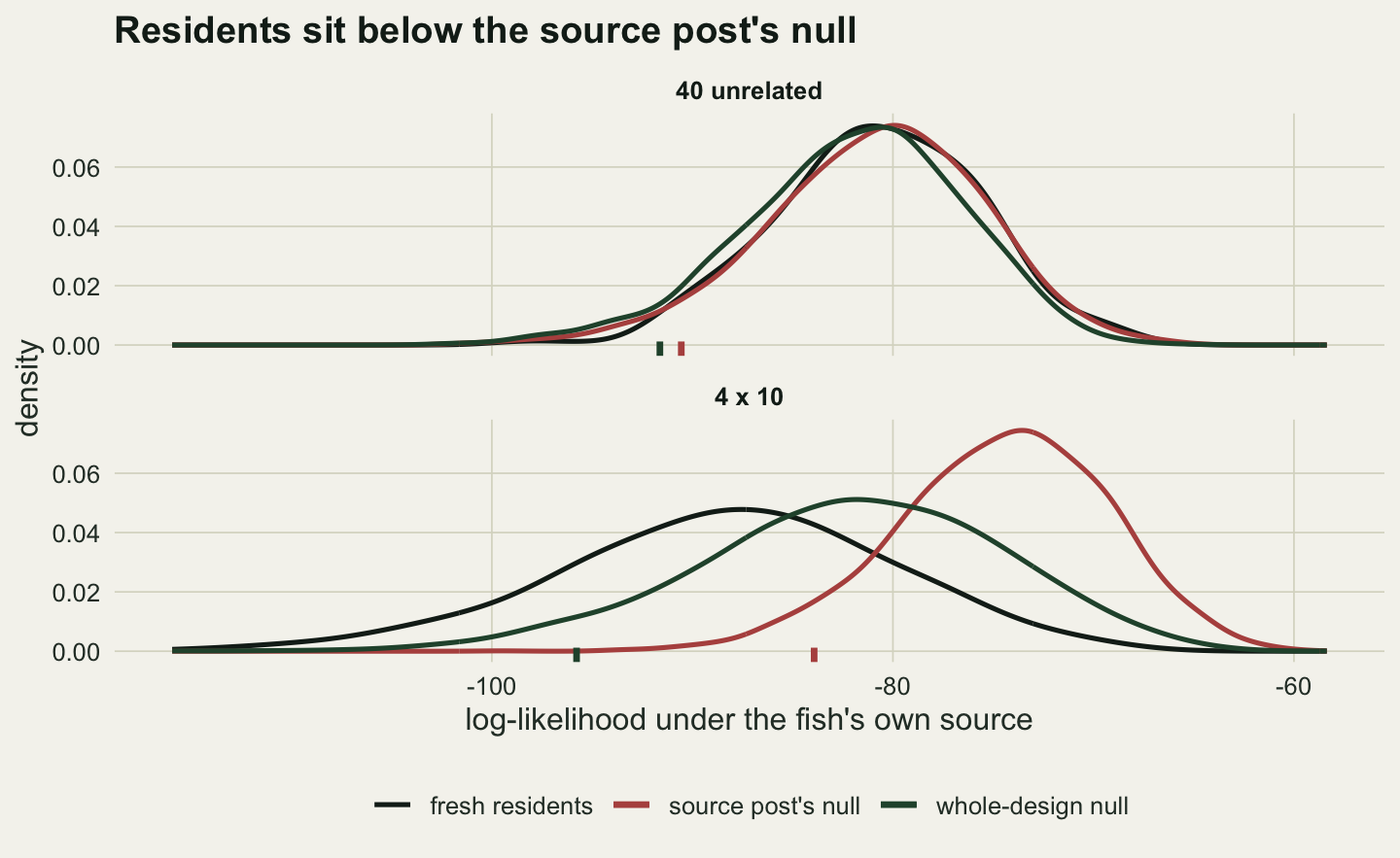
In this one example the residents fall below the source post’s 5 per cent point in 0.033 of cases with 40 unrelated fish and 0.700 with 4 families of 10; below the whole-design null’s 5 per cent point in 0.015 and 0.172.
What the repair costs, and what it needs
A null that stops excluding residents will also exclude fewer fish from the unsampled source. At a target Fst of 0.03 the exclusion test is weak whatever null is used: with 40 unrelated fish, fish from the fourth source are excluded from all three baselines in 0.195 of cases under the source post’s null and 0.151 under the whole-design null. The source post demonstrated its exclusion test at Fst = 0.1, so the chunk below repeats the grid there for three designs.
designs_high <- designs[c(1, 3, 4), c("name", "n_fam", "fam_size")]
n_sets_high <- 16
set.seed(56030)
grid_high <- run_sets(n_sets_high, 0.10, designs_high, wide = FALSE)
mh <- function(col, dsg) mean_se(grid_high, col, dsg)
high_tab <- do.call(rbind, lapply(designs_high$name, function(nm) rbind(
  data.frame(design = nm, null = "source post's null", size = mh("size_post", nm)[1],
             size_se = mh("size_post", nm)[2], power = mh("power_post", nm)[1],
             power_se = mh("power_post", nm)[2]),
  data.frame(design = nm, null = "whole-design null", size = mh("size_des", nm)[1],
             size_se = mh("size_des", nm)[2], power = mh("power_des", nm)[1],
             power_se = mh("power_des", nm)[2]))))
print(high_tab, row.names = FALSE, digits = 3)
design null size size_se power power_se
40 unrelated source post's null 0.0765 0.00510 0.834 0.02630
40 unrelated whole-design null 0.0517 0.00421 0.783 0.03072
8 x 5 source post's null 0.2715 0.01893 0.942 0.01473
8 x 5 whole-design null 0.0981 0.01183 0.823 0.02710
4 x 10 source post's null 0.5883 0.01847 0.982 0.00518
4 x 10 whole-design null 0.1365 0.01322 0.763 0.03186hv <- function(nm, nl, col) high_tab[[col]][high_tab$design == nm & high_tab$null == nl]At Fst = 0.1 the sizes stay near their values at 0.03: the source post’s null excludes 0.076, 0.271 and 0.588 of residents for 40 unrelated fish, 8 families of 5 and 4 families of 10, and the whole-design null 0.052, 0.098 and 0.136. Fish from the unsampled source are excluded from every baseline in 0.834, 0.942 and 0.982 of cases under the source post’s null, and in 0.783, 0.823 and 0.763 under the whole-design null. Part of the source post’s higher catch rate with families is bought with its excess exclusion of residents, and a catch rate from a test that also throws out 59 genuine residents in a hundred is not a catch rate that can be quoted. Under the whole-design null the catch rate changes little across the three designs.
The whole-design null asks for the number of families and their sizes. In practice those come from a sibship reconstruction, which makes errors. Both grids also scored the 8 x 5 baselines with whole-design nulls built on the wrong structure, and at Fst = 0.1 they recorded the catch rate of each of those nulls as well.
mis_cols <- c("size_as_4x10", "size_des", "size_as_20x2", "size_as_unrel")
pow_cols <- c("power_as_4x10", "power_des", "power_as_20x2", "power_as_unrel")
mis_tab <- data.frame(
  assumed = c("4 families of 10", "8 families of 5 (true)", "20 families of 2", "40 unrelated"),
  size_03 = sapply(mis_cols, function(v) ms(v, "8 x 5")[1]),
  size_10 = sapply(mis_cols, function(v) mh(v, "8 x 5")[1]),
  se_10 = sapply(mis_cols, function(v) mh(v, "8 x 5")[2]),
  catch_10 = sapply(pow_cols, function(v) mh(v, "8 x 5")[1]),
  catch_se_10 = sapply(pow_cols, function(v) mh(v, "8 x 5")[2]))
print(mis_tab, row.names = FALSE, digits = 3)
assumed size_03 size_10 se_10 catch_10 catch_se_10
4 families of 10 0.0107 0.0194 0.00298 0.534 0.0398
8 families of 5 (true) 0.0886 0.0981 0.01183 0.823 0.0271
20 families of 2 0.1825 0.1844 0.01640 0.896 0.0211
40 unrelated 0.2200 0.2250 0.01826 0.917 0.0182When the true baseline is 8 families of 5, a whole-design null that assumes 4 families of 10 excludes 0.011 of residents at Fst = 0.03 and 0.019 at 0.1; the correct structure 0.089 and 0.098; 20 families of 2 0.182 and 0.184; and no families at all 0.220 and 0.225. At Fst = 0.1 the same four nulls catch 0.534, 0.823, 0.896 and 0.917 of the fish from the unsampled source. Getting the structure wrong is a trade, not a safe side. Assuming fewer, larger families than there are keeps the size under 0.05 but gives up 35 per cent of the catches the correct structure makes; assuming more, smaller families catches a few more fish and brings much of the excess exclusion of residents back.
Self-assignment: the Ostergren result, reproduced
The same grid recorded the source post’s self-assignment rates, naive and leave-one-out, together with two alternatives: leaving the whole family out, and purging each baseline to one fish per family before leave-one-out. The truth is the rate at which the fresh residents, scored against the full baseline, go to their own source.
self_long <- do.call(rbind, lapply(designs$name, function(nm) {
  x <- grid_main[grid_main$design == nm, ]
  data.frame(design = nm,
             method = c("naive", "leave one out", "leave family out", "purge, then leave one out",
                        "fresh residents (truth)"),
             rate = c(mean(x$naive), mean(x$loo), mean(x$lfo), mean(x$purge), mean(x$truth)),
             se = c(sd(x$naive), sd(x$loo), sd(x$lfo), sd(x$purge), sd(x$truth)) / sqrt(nrow(x)))
}))
self_long <- self_long[!is.na(self_long$rate), ]
sv <- function(nm, mth) self_long$rate[self_long$design == nm & self_long$method == mth]
tr <- function(nm) mean(grid_main$truth[grid_main$design == nm])
optimism <- sapply(designs$name, function(nm) sv(nm, "leave one out") - tr(nm))
lfo_gap <- sapply(designs$name[-1], function(nm) sv(nm, "leave family out") - tr(nm))
With 40 unrelated fish, leave-one-out self-assignment reports 0.867 and fresh residents are assigned correctly 0.873 of the time, a gap of -0.007: the source post’s repair works on the baseline it was built for. With 8 families of 5, leave-one-out reports 0.974 against a truth of 0.781, and with 4 families of 10 it reports 0.998 against 0.715. Anderson, Waples and Kalinowski showed in 2008 that predicting stock identification accuracy by resampling the baseline overstates it, and replaced it with leave-one-out cross-validation, the same idea as the source post’s repair. The family rows are the pattern Ostergren and colleagues reported: the more family structure, the better the baseline looks and the worse it does.
Two things follow from the effective copies. The truth itself falls because the baseline knows less: 8 families of 5 deliver 0.781 and 13 unrelated fish 0.792; 4 families of 10 deliver 0.715 and 7 unrelated fish 0.697. And the leave-one-out rate rises because a held-out fish still has its siblings in the frequencies it is scored against.
Leaving the whole family out is the grouped version of leave-one-out. With 20 families of 2 it lands -0.001 from the truth, with 8 families of 5 -0.038, and with 4 families of 10 -0.165. With few families it is pessimistic, because holding out one family of ten removes a quarter of the source’s baseline, and what it measures is a baseline of three families. Purging to one fish per family and then leaving one out gives 0.691 and 0.465, lower again: it scores a baseline of 8 or 4 fish, not the baseline that will be used, which is the cost Waples and Anderson set out in their cautionary view of purging.
self_long$design <- factor(self_long$design, levels = rev(designs$name))
self_long$method <- factor(self_long$method, levels = c("naive", "leave one out", "leave family out",
                                                        "purge, then leave one out",
                                                        "fresh residents (truth)"))
p_self <- ggplot(self_long, aes(rate, design, colour = method, shape = method)) +
  geom_errorbar(aes(xmin = rate - 2 * se, xmax = rate + 2 * se), orientation = "y",
                width = 0.3, linewidth = 0.4, position = position_dodge(width = 0.7)) +
  geom_point(size = 2.6, position = position_dodge(width = 0.7)) +
  scale_colour_manual(values = c(te_rust, te_gold, te_forest, te_body, te_ink), name = NULL) +
  scale_shape_manual(values = c(16, 16, 17, 15, 18), name = NULL) +
  labs(x = "correct assignment rate", y = "baseline per source",
       title = "Leave-one-out flatters a family baseline") +
  guides(colour = guide_legend(nrow = 2), shape = guide_legend(nrow = 2)) +
  theme_datasheet() + theme(legend.position = "bottom")
p_self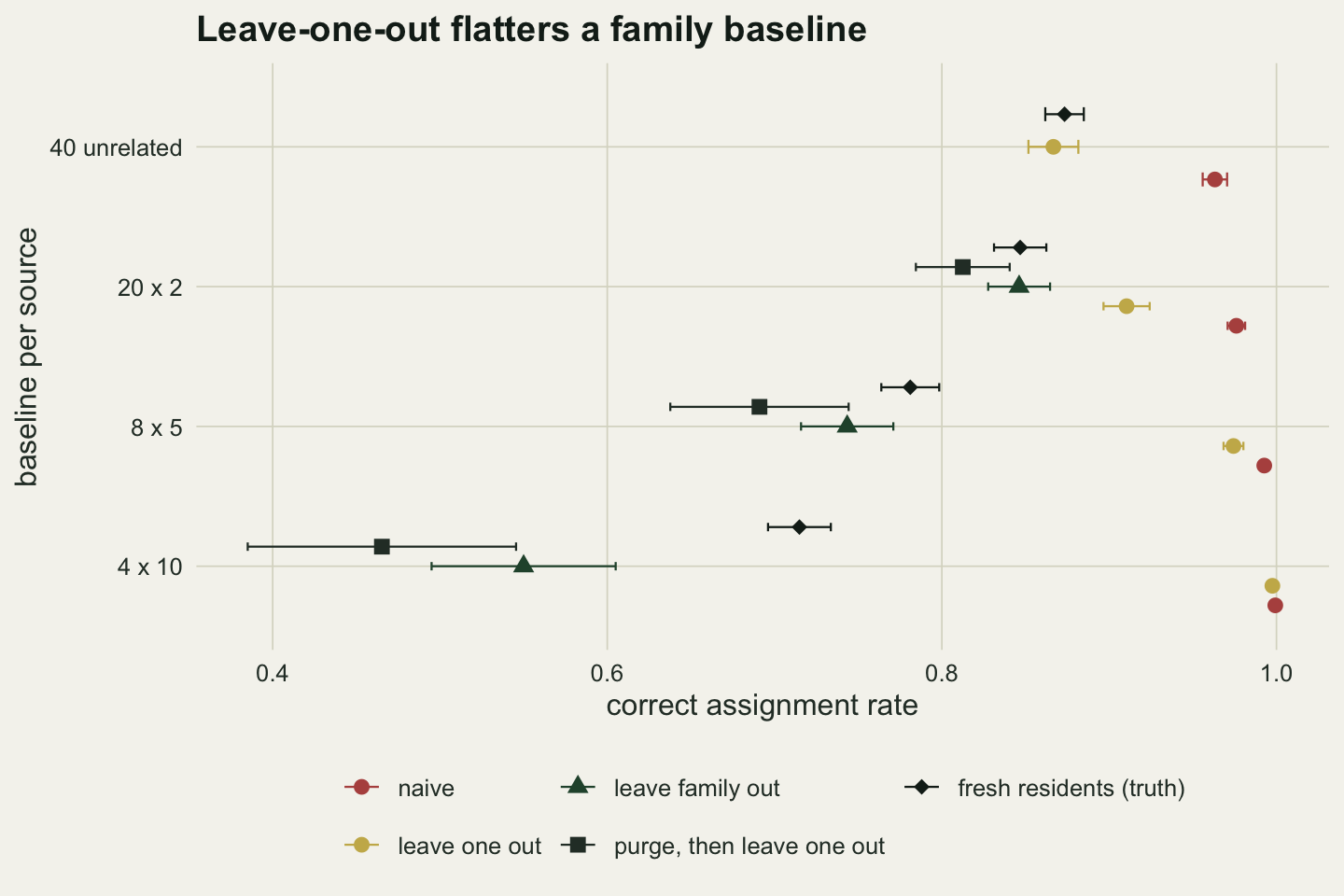
What to report
Report how the baseline was collected: the number of sites, nests or spawning riffles behind each source, and any sibship reconstruction, with the number and sizes of families it found. From those, \(m = 4FS/(S+1)\) gives the number of independent gene copies the baseline is worth for full sibs, and that number, not the head count, is what the accuracy tracks.
Do not calibrate an exclusion test on a beta posterior of the baseline frequencies when the baseline is small or built from families. In this simulation that null excluded 0.273 of genuine residents at 8 families of 5 and 0.261 with 7 unrelated fish. Simulate the whole baseline step instead, with the family structure found. When that structure is uncertain there is no safe side: in the misspecification check at Fst = 0.1, assuming too few families cut the size to 0.019 and the catch rate to 0.534 from 0.823, and assuming too many raised the size to 0.184. Report the size of the test on simulated residents alongside the exclusions it makes.
Do not report leave-one-out self-assignment from a family baseline as its accuracy; Ostergren and colleagues showed that it rises as the real accuracy falls. Leaving whole families out is close when there are many families and pessimistic when there are few, so report the number of families next to it.
Honest limits
Everything here is full sibs of equal size, unlinked loci, Hardy-Weinberg parents, and fresh residents that are unrelated to the baseline families. Half sibs share less, so they cost fewer copies; families of unequal size are worth fewer copies than equal ones of the same number, and neither was simulated; and in a real river a fresh fish can be a sibling of baseline fish, which would raise its log-likelihood rather than lower it; that case was not simulated. Only three sources, 100 biallelic loci, 40 fish per source and two levels of differentiation were simulated, with 24 sets of frequencies in the main grid and 16 at Fst = 0.1.
The whole-design null was given the true number of families and their sizes, or a structure chosen for it in the misspecification check. A sibship reconstruction from 100 biallelic loci makes errors, and how the test behaves with estimated sibships was not measured. The null also keeps an excess over 0.05 at four families of ten, and the oracle check puts it on the estimated frequencies it simulates from; drawing them from a beta posterior before simulating removed little of it, and shrinking them towards a common value across sources was not tried.
All of this is about calling single fish. Mixed-stock analysis estimates the proportions of each source in a mixture, and Ostergren and colleagues looked at those too; the proportions were not simulated here, and neither were the exclusion test’s consequences for them.
References
Anderson EC, Waples RS, Kalinowski ST 2008 Canadian Journal of Fisheries and Aquatic Sciences 65(7):1475-1486 (10.1139/F08-049)
Cornuet JM, Piry S, Luikart G, Estoup A, Solignac M 1999 Genetics 153(4):1989-2000 (10.1093/genetics/153.4.1989)
Ostergren J, Palm S, Gilbey J, Dannewitz J 2020 Molecular Ecology Resources 20(2):498-510 (10.1111/1755-0998.13131)
Waples RS, Anderson EC 2017 Molecular Ecology 26(5):1211-1224 (10.1111/mec.14022)