set.seed(4130)
tr    <- seq(1, 8, by = 1)
traps <- as.matrix(expand.grid(x = tr, y = tr)); J <- nrow(traps)
K     <- 6
a0_true <- qlogis(0.18); a1_true <- 1.1; sig_true <- 0.75
buffer  <- 3
xl <- range(traps[, 1]) + c(-buffer, buffer); yl <- range(traps[, 2]) + c(-buffer, buffer)
A  <- diff(xl) * diff(yl); N_true <- 90; D_true <- N_true / A

effort <- rnorm(J)                                   # standardised effort per trap
g0_j   <- plogis(a0_true + a1_true * effort)

sx <- runif(N_true, xl[1], xl[2]); sy <- runif(N_true, yl[1], yl[2])
d2 <- outer(sx, traps[, 1], "-")^2 + outer(sy, traps[, 2], "-")^2
P  <- sweep(exp(-d2 / (2 * sig_true^2)), 2, g0_j, "*")
Yf <- matrix(rbinom(N_true * J, K, P), N_true, J)
cc <- rowSums(Yf) > 0; Y <- Yf[cc, , drop = FALSE]; n <- nrow(Y)
trap_tot <- colSums(Y)Detection covariates and checking in SCR
R
capture-recapture
spatial
model diagnostics
ecology tutorial
Add a trap-effort covariate to the SCR detection function in base R, and use a parametric-bootstrap goodness-of-fit that a constant-detection model fails.
Detection in a spatial capture-recapture study is rarely uniform across traps. Some detectors run longer, sit in better habitat, or use more attractive lures, so their baseline detection g0 differs. Ignore that and two things happen: the detection model is wrong, and the wrongness can leak into density. This post adds a trap-level effort covariate to the SCR detection function, fits it from scratch, and then does the part that is easy to skip: checking whether the fitted detection model actually reproduces the data, using a parametric bootstrap. A model that ignores effort passes every casual glance but fails the check; the model with effort passes.
Effort on the baseline detection
We keep the half-normal distance kernel but let the baseline detection depend on a trap-level covariate through a logit link:
\[g_{0j} = \operatorname{logit}^{-1}(a_0 + a_1 \, \text{effort}_j), \qquad p_{ij}(s) = g_{0j}\, \exp\!\left(-\frac{d(s, x_j)^2}{2\sigma^2}\right).\]
Each trap j carries its own baseline g0j; high-effort traps detect more. Everything else (the activity-centre integral, the Poisson point process for density) is unchanged from the basics post.
The study catches 49 animals with 208 detections and 39 spatial recaptures.
Two detection models
We fit two versions of the same integrated likelihood: a null model with a single constant g0, and a full model where g0 depends on effort.
gx <- seq(xl[1], xl[2], length.out = 35); gy <- seq(yl[1], yl[2], length.out = 35)
G  <- as.matrix(expand.grid(x = gx, y = gy))
d2G <- outer(G[, 1], traps[, 1], "-")^2 + outer(G[, 2], traps[, 2], "-")^2
Cc  <- rowSums(lchoose(K, Y))

nll_null <- function(th) {                           # logD, qlogis g0, log sigma
  Dd <- exp(th[1]); g0 <- plogis(th[2]); sg <- exp(th[3])
  Pg <- g0 * exp(-d2G / (2 * sg^2))
  pb <- mean(1 - exp(rowSums(K * log1p(-Pg)))); if (pb <= 0) return(1e10)
  LM <- Y %*% t(log(Pg)) + (K - Y) %*% t(log1p(-Pg)) + Cc
  m  <- apply(LM, 1, max); lf <- m + log(rowMeans(exp(LM - m)))
  -(dpois(n, Dd * A * pb, log = TRUE) + sum(lf) - n * log(pb))
}
nll_full <- function(th) {                           # logD, a0, a1, log sigma
  Dd <- exp(th[1]); gj <- plogis(th[2] + th[3] * effort); sg <- exp(th[4])
  Pg <- sweep(exp(-d2G / (2 * sg^2)), 2, gj, "*")
  pb <- mean(1 - exp(rowSums(K * log1p(-Pg)))); if (pb <= 0) return(1e10)
  LM <- Y %*% t(log(Pg)) + (K - Y) %*% t(log1p(-Pg)) + Cc
  m  <- apply(LM, 1, max); lf <- m + log(rowMeans(exp(LM - m)))
  -(dpois(n, Dd * A * pb, log = TRUE) + sum(lf) - n * log(pb))
}
f0 <- optim(c(log(n/(A*0.4)), qlogis(0.18), log(0.8)), nll_null,
            method = "BFGS", hessian = TRUE, control = list(maxit = 500, reltol = 1e-10))
f1 <- optim(c(log(n/(A*0.4)), a0_true, 1.0, log(0.8)), nll_full,
            method = "BFGS", hessian = TRUE, control = list(maxit = 500, reltol = 1e-10))
a1h <- f1$par[3]; se1 <- sqrt(diag(solve(f1$hessian)))
aic0 <- 2*f0$value + 2*length(f0$par); aic1 <- 2*f1$value + 2*length(f1$par)
lrt  <- 2*(f0$value - f1$value); lrt_p <- pchisq(lrt, 1, lower.tail = FALSE)
D0 <- exp(f0$par[1]); g0_0 <- plogis(f0$par[2]); sig0 <- exp(f0$par[3])
D1 <- exp(f1$par[1]); sig1 <- exp(f1$par[4])
The full model recovers the effort effect (a1 estimated at 1.014 with standard error 0.14, against the true 1.1) and is strongly preferred: the likelihood-ratio statistic is 71.7 on one degree of freedom (p below 2.5^{-17}), and the effort model has an AIC lower by 69.7. Both models return almost the same density (0.583 null, 0.58 full), so on density alone you might never notice the null model is wrong. That is exactly why a fit check matters.
Does the detection model fit?
A parametric-bootstrap goodness-of-fit test asks whether a summary of the data is reproducible by the fitted model. The natural summary for a detection covariate is the correlation between each trap’s total detections and its effort. Simulate many datasets from a fitted model, compute the statistic each time, and see where the observed value falls.
Tstat <- function(Ymat) cor(colSums(Ymat), effort)
T_obs <- Tstat(Y)

sim_data <- function(D, sg, gj) {                    # gj is the trap-level g0 vector
  Ns <- rpois(1, D * A)
  xs <- runif(Ns, xl[1], xl[2]); ys <- runif(Ns, yl[1], yl[2])
  d2s <- outer(xs, traps[, 1], "-")^2 + outer(ys, traps[, 2], "-")^2
  Yz  <- matrix(rbinom(Ns * J, K, sweep(exp(-d2s / (2 * sg^2)), 2, gj, "*")), Ns, J)
  Yz[rowSums(Yz) > 0, , drop = FALSE]
}
set.seed(77)
B  <- 500
T0 <- replicate(B, Tstat(sim_data(D0, sig0, rep(g0_0, J))))               # null model
T1 <- replicate(B, Tstat(sim_data(D1, sig1, plogis(f1$par[2] + a1h * effort))))  # full model
p0 <- mean(T0 >= T_obs); p1 <- mean(T1 >= T_obs)
The observed correlation between trap totals and effort is 0.535. Under the constant-detection model it should be near zero, and it is: the null model’s simulated correlations centre on 0.003 and the observed value falls far in the upper tail (p = 0), a clear failure. Under the effort model the simulated correlations centre on 0.616 and the observed value sits comfortably inside (p = 0.834). Same density from both models, but only one reproduces how detections are distributed across traps.
td <- data.frame(effort = effort, total = trap_tot)
p1p <- ggplot(td, aes(effort, total)) +
  geom_hline(yintercept = mean(trap_tot), colour = rust, linetype = "dashed", linewidth = 0.7) +
  geom_smooth(method = "lm", se = FALSE, colour = forest, linewidth = 0.9) +
  geom_point(colour = ink, size = 2, alpha = 0.8) +
  annotate("text", x = min(effort), y = mean(trap_tot), label = "constant-g0 prediction",
           vjust = -0.7, hjust = 0, colour = rust, size = 3.2) +
  labs(x = "trap effort (standardised)", y = "total detections at trap",
       title = "High-effort traps detect more",
       subtitle = "the constant-detection model has no way to represent this") +
  theme_te()
p1p
`geom_smooth()` using formula = 'y ~ x'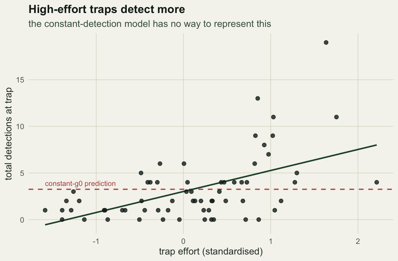
gof <- rbind(data.frame(stat = T0, model = "constant g0"),
             data.frame(stat = T1, model = "effort on g0"))
labs_df <- data.frame(model = c("constant g0", "effort on g0"),
                      lab = c(paste0("p = ", round(p0, 3)), paste0("p = ", round(p1, 3))))
p2p <- ggplot(gof, aes(stat)) +
  geom_histogram(bins = 34, fill = sage, colour = paper, linewidth = 0.2) +
  geom_vline(xintercept = T_obs, colour = ink, linewidth = 0.8) +
  geom_text(data = labs_df, aes(x = -Inf, y = Inf, label = lab),
            hjust = -0.2, vjust = 1.6, colour = ink, size = 3.4, inherit.aes = FALSE) +
  facet_wrap(~ model, scales = "free_x") +
  labs(x = "correlation of trap totals with effort", y = "simulated datasets",
       title = "Only the effort model reproduces the data",
       subtitle = "observed value (line) in the tail for constant g0, inside for effort") +
  theme_te()
p2p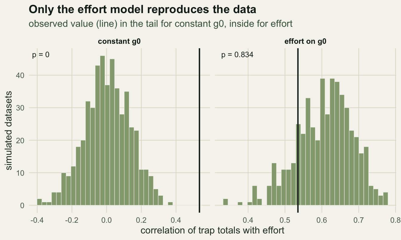
Takeaways
Detection covariates belong in the SCR detection function whenever effort or conditions vary across traps, and adding one is a small change: the baseline g0 becomes a logit-linear function of the covariate inside the same likelihood. The subtler point is that density can look fine while the detection model is wrong, so a fit check is not optional. A parametric bootstrap makes it concrete: pick a statistic the covariate should affect (here the trap-total to effort correlation), simulate from the fitted model, and see whether the observed value is reproducible. The constant-detection model fails that test decisively while giving a plausible density; the effort model passes. This closes the spatial capture-recapture series: estimate density, do it the Bayesian way, design the array, and check the detection model that everything rests on.
References
Borchers, D. L. and Efford, M. G. 2008. Spatially explicit maximum likelihood methods for capture-recapture studies. Biometrics 64(2):377-385 (10.1111/j.1541-0420.2007.00927.x).
Efford, M. G., Borchers, D. L. and Byrom, A. E. 2009. Density estimation by spatially explicit capture-recapture: likelihood-based methods. In: Modeling Demographic Processes in Marked Populations, Springer (10.1007/978-0-387-78151-8_11).
Royle, J. A., Karanth, K. U., Gopalaswamy, A. M. and Kumar, N. S. 2009. Bayesian inference in camera trapping studies for a class of spatial capture-recapture models. Ecology 90(11):3233-3244 (10.1890/08-1481.1).
Efford, M. 2004. Density estimation in live-trapping studies. Oikos 106(3):598-610 (10.1111/j.0030-1299.2004.13043.x).
Royle, J. A., Chandler, R. B., Sollmann, R. and Gardner, B. 2014. Spatial Capture-Recapture. Academic Press (ISBN 978-0-12-405939-9).